Lecture Notes on Compositional Data Analysis - Sedimentology ...

42 Chapter 5. Exploratory data analysis
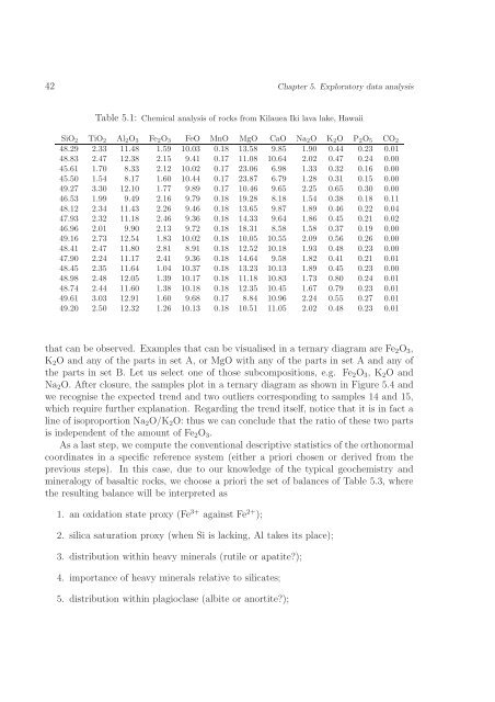
Table 5.1: Chemical analysis of rocks from Kilauea Iki lava lake, Hawaii
SiO 2 TiO 2 Al 2 O 3 Fe 2 O 3 FeO MnO MgO CaO Na 2 O K 2 O P 2 O 5 CO 2
48.29 2.33 11.48 1.59 10.03 0.18 13.58 9.85 1.90 0.44 0.23 0.01
48.83 2.47 12.38 2.15 9.41 0.17 11.08 10.64 2.02 0.47 0.24 0.00
45.61 1.70 8.33 2.12 10.02 0.17 23.06 6.98 1.33 0.32 0.16 0.00
45.50 1.54 8.17 1.60 10.44 0.17 23.87 6.79 1.28 0.31 0.15 0.00
49.27 3.30 12.10 1.77 9.89 0.17 10.46 9.65 2.25 0.65 0.30 0.00
46.53 1.99 9.49 2.16 9.79 0.18 19.28 8.18 1.54 0.38 0.18 0.11
48.12 2.34 11.43 2.26 9.46 0.18 13.65 9.87 1.89 0.46 0.22 0.04
47.93 2.32 11.18 2.46 9.36 0.18 14.33 9.64 1.86 0.45 0.21 0.02
46.96 2.01 9.90 2.13 9.72 0.18 18.31 8.58 1.58 0.37 0.19 0.00
49.16 2.73 12.54 1.83 10.02 0.18 10.05 10.55 2.09 0.56 0.26 0.00
48.41 2.47 11.80 2.81 8.91 0.18 12.52 10.18 1.93 0.48 0.23 0.00
47.90 2.24 11.17 2.41 9.36 0.18 14.64 9.58 1.82 0.41 0.21 0.01
48.45 2.35 11.64 1.04 10.37 0.18 13.23 10.13 1.89 0.45 0.23 0.00
48.98 2.48 12.05 1.39 10.17 0.18 11.18 10.83 1.73 0.80 0.24 0.01
48.74 2.44 11.60 1.38 10.18 0.18 12.35 10.45 1.67 0.79 0.23 0.01
49.61 3.03 12.91 1.60 9.68 0.17 8.84 10.96 2.24 0.55 0.27 0.01
49.20 2.50 12.32 1.26 10.13 0.18 10.51 11.05 2.02 0.48 0.23 0.01
that can be observed. Examples that can be visualised in a ternary diagram are Fe 2 O 3 ,
K 2 O and any of the parts in set A, or MgO with any of the parts in set A and any of
the parts in set B. Let us select one of those subcompositions, e.g. Fe 2 O 3 , K 2 O and
Na 2 O. After closure, the samples plot in a ternary diagram as shown in Figure 5.4 and
we recognise the expected trend and two outliers corresponding to samples 14 and 15,
which require further explanation. Regarding the trend itself, notice that it is in fact a
line of isoproportion Na 2 O/K 2 O: thus we can conclude that the ratio of these two parts
is independent of the amount of Fe 2 O 3 .
As a last step, we compute the conventional descriptive statistics of the orthonormal
coordinates in a specific reference system (either a priori chosen or derived from the
previous steps). In this case, due to our knowledge of the typical geochemistry and
mineralogy of basaltic rocks, we choose a priori the set of balances of Table 5.3, where
the resulting balance will be interpreted as
1. an oxidation state proxy (Fe 3+ against Fe 2+ );
2. silica saturation proxy (when Si is lacking, Al takes its place);
3. distribution within heavy minerals (rutile or apatite?);
4. importance of heavy minerals relative to silicates;
5. distribution within plagioclase (albite or anortite?);