Lecture Notes on Compositional Data Analysis - Sedimentology ...

36 Chapter 5. Exploratory data analysis
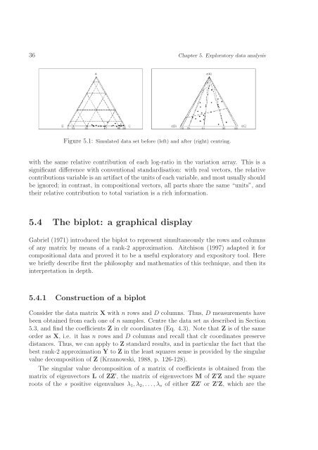
Figure 5.1: Simulated data set before (left) and after (right) centring.
with the same relative contribution of each log-ratio in the variation array. This is a
significant difference with conventional standardisation: with real vectors, the relative
contributions variable is an artifact of the units of each variable, and most usually should
be ignored; in contrast, in compositional vectors, all parts share the same “units”, and
their relative contribution to total variation is a rich information.
5.4 The biplot: a graphical display
Gabriel (1971) introduced the biplot to represent simultaneously the rows and columns
of any matrix by means of a rank-2 approximation. Aitchison (1997) adapted it for
compositional data and proved it to be a useful exploratory and expository tool. Here
we briefly describe first the philosophy and mathematics of this technique, and then its
interpretation in depth.
5.4.1 Construction of a biplot
Consider the data matrix X with n rows and D columns. Thus, D measurements have
been obtained from each one of n samples. Centre the data set as described in Section
5.3, and find the coefficients Z in clr coordinates (Eq. 4.3). Note that Z is of the same
order as X, i.e. it has n rows and D columns and recall that clr coordinates preserve
distances. Thus, we can apply to Z standard results, and in particular the fact that the
best rank-2 approximation Y to Z in the least squares sense is provided by the singular
value decomposition of Z (Krzanowski, 1988, p. 126-128).
The singular value decomposition of a matrix of coefficients is obtained from the
matrix of eigenvectors L of ZZ ′ , the matrix of eigenvectors M of Z ′ Z and the square
roots of the s positive eigenvalues λ 1 , λ 2 , . . .,λ s of either ZZ ′ or Z ′ Z, which are the