Lecture Notes on Compositional Data Analysis - Sedimentology ...

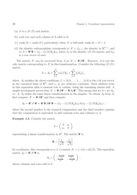
30 Chapter 4. Coordinate representation
(a) it is a (D, D) real matrix;
(b) each row and each column of A adds to 0;
(c) rank(A) = rank(A ∗ ); particularly, when A ∗ is full-rank, rank(A) = D − 1;
(d) the identity endomorphism corresponds to A ∗ = I D−1 , the identity in R D−1 , and
to A = Ψ ′ Ψ = I D − (1/D)1 ′ D 1 D, where I D is the identity (D, D)-matrix, and 1 D
is a row vector of ones.
The matrix A ∗ can be recovered from A as A ∗ = ΨAΨ ′ . However, A is not the
only matrix corresponding to A ∗ in this transformation. Consider the following (D, D)-
matrix
D∑
D∑
A = A 0 + c i (⃗e i ) ′ 1 D + d j 1 ′ D⃗e j ,
i=1
where, A 0 satisfies the above conditions, ⃗e i = [0, 0, . . ., 1, . . ., 0, 0] is the i-th row-vector
in the canonical basis of R D , and c i , d j are arbitrary constants. Each additive term
in this expression adds a constant row or column, being the remaining entries null. A
simple development proves that A ∗ = ΨAΨ ′ = ΨA 0 Ψ ′ . This means that x◦A = x◦A 0 ,
i.e. A, A 0 define the same linear transformation in the simplex. To obtain A 0 from A,
first compute A ∗ = ΨAΨ ′ and then compute
A 0 = Ψ ′ A ∗ Ψ = Ψ ′ ΨAΨ ′ Ψ = (I D − (1/D)1 ′ D 1 D)A(I D − (1/D)1 ′ D 1 D) ,
where the second member is the required computation and the third member explains
that the computation is equivalent to add constant rows and columns to A.
j=1
Example 4.3. Consider the matrix
A =
(
0 a2
a 1 0
)
representing a linear transformation in S 2 . The matrix Ψ is
[ 1√2
Ψ = , −√ 1 ]
.
2
In coordinates, this corresponds to a (1, 1)-matrix A ∗ = (−(a1+a2)/2). The equivalent
matrix A 0 = Ψ ′ A ∗ Ψ is ( −
a 1 +a 2 a 1 +a 2
)
A 0 =
4 4
,
whose columns and rows add to 0.
a 1 +a 2
− a 1+a 2
4 4