Lecture Notes on Compositional Data Analysis - Sedimentology ...

More documents

Recommendations

Info

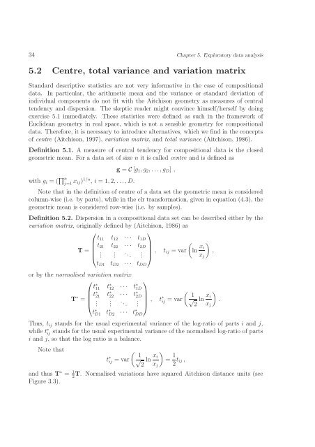
34 Chapter 5. Exploratory data analysis 5.2 Centre, total variance and variation matrix Standard descriptive statistics are not very informative in the case of compositional data. In particular, the arithmetic mean and the variance or standard deviation of individual components do not fit with the Aitchison geometry as measures of central tendency and dispersion. The skeptic reader might convince himself/herself by doing exercise 5.1 immediately. These statistics were defined as such in the framework of Euclidean geometry in real space, which is not a sensible geometry for compositional data. Therefore, it is necessary to introduce alternatives, which we find in the concepts of centre (Aitchison, 1997), variation matrix, and total variance (Aitchison, 1986). Definition 5.1. A measure of central tendency for compositional data is the closed geometric mean. For a data set of size n it is called centre and is defined as with g i = ( ∏ n j=1 x ij) 1/n , i = 1, 2, . . ., D. g = C [g 1 , g 2 , . . .,g D ] , Note that in the definition of centre of a data set the geometric mean is considered column-wise (i.e. by parts), while in the clr transformation, given in equation (4.3), the geometric mean is considered row-wise (i.e. by samples). Definition 5.2. Dispersion in a compositional data set can be described either by the variation matrix, originally defined by (Aitchison, 1986) as ⎛ ⎞ t 11 t 12 · · · t 1D t 21 t 22 · · · t 2D ( T = ⎜ ⎝ . . . .. ⎟ . ⎠ , t ij = var ln x ) i , x j t D1 t D2 · · · t DD or by the normalised variation matrix ⎛ ⎞ t ∗ 11 t ∗ 12 · · · t ∗ 1D T ∗ t ∗ 21 t ∗ 22 · · · t ∗ ( 2D 1 = ⎜ ⎝ . . .. ⎟ . . ⎠ , t∗ ij = var √2 ln x ) i . x j t ∗ D1 t ∗ D2 · · · t ∗ DD Thus, t ij stands for the usual experimental variance of the log-ratio of parts i and j, while t ∗ ij stands for the usual experimental variance of the normalised log-ratio of parts i and j, so that the log ratio is a balance. Note that t ∗ ij = var ( 1 √2 ln x i x j ) = 1 2 t ij , and thus T ∗ = 1 2 T. Normalised variations have squared Aitchison distance units (see Figure 3.3).
5.3 Centring and scaling 35 Definition 5.3. A measure of global dispersion is the total variance given by totvar[X] = 1 2D D∑ i=1 D∑ j=1 ( var ln x ) i = 1 x j 2D D∑ i=1 D∑ t ij = 1 D j=1 D∑ i=1 D∑ t ∗ ij . By definition, T and T ∗ are symmetric and their diagonal will contain only zeros. Furthermore, neither the total variance nor any single entry in both variation matrices depend on the constant κ associated with the sample space S D , as constants cancel out when taking ratios. Consequently, rescaling has no effect. These statistics have further connections. From their definition, it is clear that the total variation summarises the variation matrix in a single quantity, both in the normalised and non-normalised version, and it is possible (and natural) to define it because all parts in a composition share a common scale (it is by no means so straightforward to define a total variation for a pressure-temperature random vector, for instance). Conversely, the variation matrix, again in both versions, explains how the total variation is split among the parts (or better, among all log-ratios). j=1 5.3 Centring and scaling A usual way in geology to visualise data in a ternary diagram is to rescale the observations in such a way that their range is approximately the same. This is nothing else but applying a perturbation to the data set, a perturbation which is usually chosen by trial and error. To overcome this somehow arbitrary approach, note that, as mentioned in Proposition 3.1, for a composition x and its inverse x −1 it holds that x ⊕ x −1 = n, the neutral element. This means that we can move by perturbation any composition to the barycentre of the simplex, in the same way we move real data in real space to the origin by translation. This property, together with the definition of centre, allows us to design a strategy to better visualise the structure of the sample. To do that, we just need to compute the centre g of our sample, as in Definition 5.1, and perturb the sample by the inverse g −1 . This has the effect of moving the centre of a data set to the barycentre of the simplex, and the sample will gravitate around the barycentre. This property was first introduced by Martín-Fernández et al. (1999) and used by Buccianti et al. (1999). An extensive discussion can be found in von Eynatten et al. (2002), where it is shown that a perturbation transforms straight lines into straight lines. This allows the inclusion of gridlines and compositional fields in the graphical representation without the risk of a nonlinear distortion. See Figure 5.1 for an example of a data set before and after perturbation with the inverse of the closed geometric mean and the effect on the gridlines. In the same way in real space one can scale a centred variable dividing it by the standard deviation, we can scale a (centred) compositional data set X by powering it with 1/ √ totvar[X]. In this way, we obtain a data set with unit total variance, but
Page 1 and 2: Lecture No
Page 3 and 4: Preface These notes have been prepa
Page 5 and 6: Contents Preface i 1 Introduction 1
Page 7 and 8: Chapter 1 Introduction The awarenes
Page 9 and 10: 3 centred logratio transformation (
Page 11 and 12: Chapter 2 Compositional data and th
Page 13 and 14: 2.2 Principles of compositional ana
Page 15 and 16: 2.3 Exercises 9 Definition 2.6. a f
Page 17 and 18: Chapter 3 The Aitchison geometry 3.
Page 19 and 20: 3.3 Inner product, norm and distanc
Page 21 and 22: 3.4. GEOMETRIC FIGURES 15 3.4 Geome
Page 23 and 24: Chapter 4 Coordinate representation
Page 25 and 26: 4.3. Generating systems 19 where (
Page 27 and 28: 4.4 Orthonormal coordinates 21 been
Page 29 and 30: 4.4 Orthonormal coordinates 23 Exam
Page 31 and 32: 4.5. WORKING IN COORDINATES 25 4.5
Page 33 and 34: 4.6. Additive log-ratio coordinates
Page 35 and 36: 4.7. Matrix notation 29 In coordina
Page 37 and 38: 4.8. EXERCISES 31 4.8 Exercises Exe
Page 39: Chapter 5 Exploratory data analysis
Page 43 and 44: 5.4. The biplot 37 same. As a resul
Page 45 and 46: 5.5. EXPLORATORY ANALYSIS OF COORDI
Page 47 and 48: 5.6. Illustration 41 0.00 0.02 0.04
Page 49 and 50: 5.6. Illustration 43 Table 5.2: Nor
Page 51 and 52: 5.6. Illustration 45 Figure 5.4: Pl
Page 53 and 54: 5.7. Exercises 47 Table 5.4: Covari
Page 55 and 56: Chapter 6 Distributions on the simp
Page 57 and 58: 6.3. Tests of normality 51 which is
Page 59 and 60: 6.3. Tests of normality 53 Tolosana
Page 61 and 62: 6.4. Exercises 55 Table 6.3: Critic
Page 63 and 64: Chapter 7 Statistical inference 7.1
Page 65 and 66: 7.1. Hypothesis about two groups 59
Page 67 and 68: 7.2. Probability and confidence reg
Page 69 and 70: Chapter 8 Compositional processes C
Page 71 and 72: 8.1. Linear processes 65 x1 2 t=0 1
Page 73 and 74: 8.2. Complementary processes 67 Exa
Page 75 and 76: 8.2. Complementary processes 69 0.5
Page 77 and 78: 8.3. Mixture processes 71 Example 8
Page 79 and 80: 8.4. Linear regression with composi
Page 81 and 82: 8.5. PRINCIPAL COMPONENT ANALYSIS 7
Page 83 and 84: 8.5. Principal component analysis 7
Page 85 and 86: 8.5. Principal component analysis 7
Page 87 and 88: Bibliography Aitchison, J. (1981).
Page 89 and 90: BIBLIOGRAPHY 83 Buccianti, A., V. P
Page 91 and 92:
BIBLIOGRAPHY 85 study of surface wa
Page 93 and 94:
A. Plotting a ternary diagram Denot
Page 95 and 96:
B. Parametrisation of an elliptic r
show all

Lecture Notes on Compositional Data Analysis - Sedimentology ...

Create successful ePaper yourself

Delete template?

Save as template?