Additional Homework Problems - Pearson

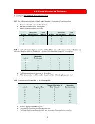
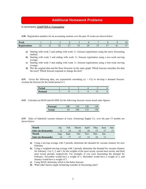
to accompany CHAPTER 4: Forecasting
Additional Homework Problems
4.50 Registration numbers for an accounting seminar over the past 10 weeks are shown below:
Week 1 2 3 4 5 6 7 8 9 10
Registrations 22 21 25 27 35 29 33 37 41 37
a) Starting with week 2 and ending with week 11, forecast registrations using the naive forecasting
method.
b) Starting with week 3 and ending with week 11, forecast registration using a two-week moving
average.
c) Starting with week 5 and ending with week 11, forecast registrations using a four-week moving
average.
d) Plot the original data and the three forecasts on the same graph. Which forecast smoothes the data
the most? Which forecast responds to change the best?
4.51 Given the following data, use exponential smoothing ( = 0.2) to develop a demand forecast.
Assume the forecast for the initial period is 5.
Period 1 2 3 4 5 6
Demand 7 9 5 9 13 8
4.52 Calculate (a) MAD and (b) MSE for the following forecast versus actual sales figures:
Forecast 100 110 120 130
Actual 95 108 123 130
4.53 Sales of industrial vacuum cleaners at Larry Armstrong Supply Co. over the past 13 months are
shown below:
Month Jan. Feb. March April May June July
Sales (in thousands) 11 14 16 10 15 17 11
Month Aug. Sept. Oct. Nov. Dec. Jan.
Sales (in thousands) 14 17 12 14 16 11
a) Using a moving average with 3 periods, determine the demand for vacuum cleaners for next
February.
b) Using a weighted moving average with 3 periods, determine the demand for vacuum cleaners
for February. Use 3, 2, and 1 for the weights of the most recent, second most recent, and third
most recent periods, respectively. For example, if you were forecasting the demand for
February, November would have a weight of 1, December would have a weight of 2, and
January would have a weight of 3.
c) Using MAD, determine which is the better forecast.
d) What other factors might Armstrong consider in forecasting sales?
1

4.54 Passenger miles flown on Northeast Airlines, a commuter firm serving the Boston hub, are shown for
the past 12 weeks:
Week 1 2 3 4 5 6 7 8 9 10 11 12
Actual Passenger
Miles (in thousands) 17 21 19 23 18 16 20 18 22 20 15 22
a) Assuming an initial forecast for week 1 of 17,000 miles, use exponential smoothing to
compute miles for weeks 2 through 12. Use α = .2.
b) What is the MAD for this model?
c) Compute the Cumulative Forecast Errors and tracking signals. Are they within acceptable
limits?
4.55 Given the following data, use least squares regression to derive a trend equation. What is your
estimate of the demand in period 7? In period 12?
Period 1 2 3 4 5 6
Demand 7 9 5 11 10 13
4.56 Joe Barrow, owner of Barrow’s Department Store, has used time-series extrapolation to forecast
retail sales for the next 4 quarters. The sales estimates are $120,000, $140,000, $160,000, and $180,000 for
the respective quarters. Seasonal indices for the 4 quarters have been found to be 1.25, .90, .75, and 1.10,
respectively. Compute a seasonalized or adjusted sales forecast.
4.57 The director of the Riley County, Kansas, library system would like to forecast evening patron usage
for next week. Below are the data for the past 4 weeks:
Mon Tue Wed Thu Fri Sat
Week 1 210 178 250 215 160 180
Week 2 215 180 250 213 165 185
Week 3 220 176 260 220 175 190
Week 4 225 178 260 225 176 190
a) Calculate a seasonal index for each day of the week.
b) If the trend equation for this problem is ŷ= 201.74 + .18x, what is the forecast for each day of
week 5? Round your forecast to the nearest whole number.
2

4.58 A careful analysis of the cost of operating an automobile was conducted by a firm. The following
model was developed:
ŷ = 4,000 + 0.20x
Where
ŷ is the annual cost and x is the miles driven.
a) If the car is driven 15,000 miles this year, what is the forecasted cost of operating this automobile?
b) If the car is driven 25,000 miles this year, what is the forecasted cost of operating this automobile?
4.59 The following multiple-regression model was developed to predict job performance as measured by a
company job performance evaluation index based on a preemployment test score and college grade point
average (GPA):
Where
ŷ = 35 + 20x 1 + 50x 2
ŷ = job performance evaluation index
x 1 = preemployment test score
x 2 = college GPA
a) Forecast the job performance index for an applicant who had a 3.0 GPA and scored 80 on the
preemployment test.
b) Forecast the job performance index for an applicant who had a 2.5 GPA and scored 70 on the
preemployment test.
4.60 A study to determine the correlation between bank deposits and consumer price indices in
Birmingham, Alabama, revealed the following (which was based on n = 5 years of data):
‣ x = 15
‣ x 2 = 55
‣ xy = 70
‣ y = 20
‣ y 2 = 130
a) What is the equation of the least square regression line?
b) Find the coefficient of correlation. What does it imply to you?
c) What is the standard error of the estimate?
3

4.61 The accountant at Rick Wing Coal Distributors, Inc., in San Francisco notes that the demand for coal
seems to be tied to an index of weather severity developed by the U.S. Weather Bureau. When weather was
extremely cold in the U.S. over the past 5 years (and the index was thus high), coal sales were high. The
accountant proposes that one good forecast of next year’s coal demand could be made by developing a
regression equation and then consulting the Farmer’s Almanac to see how severe next year’s winter would
be. For the data in the following table, derive a least squares regression and compute the coefficient of
correlation of the data. Also compute the standard error of the estimate.
Coal Sales (in millions of tons), y 4 1 4 6 5
Weather Index, x 2 1 4 5 3
4.62 Given the following data, use least squares regression to develop a relation between the number of
rainy summer days and the number of games lost by the Boca Raton Cardinal baseball team.
Years 2001 2002 2003 2004 2005 2006 2007 2008 2009 2010
Rainy Days 15 25 10 10 30 20 20 15 10 25
Games Lost 25 20 10 15 20 15 20 10 5 20
4