Stochastic Volatility and Seasonality in ... - Interconti, Limited
Stochastic Volatility and Seasonality in ... - Interconti, Limited
Stochastic Volatility and Seasonality in ... - Interconti, Limited

You also want an ePaper? Increase the reach of your titles
YUMPU automatically turns print PDFs into web optimized ePapers that Google loves.
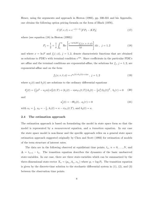
Hence, us<strong>in</strong>g the arguments <strong>and</strong> approach <strong>in</strong> Heston (1993), pp. 330-331 <strong>and</strong> his Appendix,<br />
one obta<strong>in</strong>s the follow<strong>in</strong>g option pric<strong>in</strong>g formula on the form of Black (1976),<br />
C(F, v, t) = e −r(τ−t) [F P 1 − KP 2 ] (17)<br />
where (see equation (18) <strong>in</strong> Heston (1993))<br />
P j = 1 2 + 1 ∫ [<br />
]<br />
∞<br />
e −iφ ln[K] f j (x, v, t; φ)<br />
Re<br />
dφ , j = 1, 2 (18)<br />
π<br />
iφ<br />
0<br />
<strong>and</strong> where x = ln F <strong>and</strong> f j (·; φ), j = 1, 2, denote characteristic functions that are obta<strong>in</strong>ed<br />
as solutions to PDE’s with term<strong>in</strong>al condition e iφx . S<strong>in</strong>ce coefficients <strong>in</strong> the particular PDE’s<br />
are aff<strong>in</strong>e <strong>and</strong> the term<strong>in</strong>al conditions are exponential-aff<strong>in</strong>e, the solutions for f j , j = 1, 2, are<br />
exponential-aff<strong>in</strong>e <strong>and</strong> on the form<br />
f j (x, v, t; φ) = e a j(t)+b j (t)v+iφx , j = 1, 2 (19)<br />
where a j (t) <strong>and</strong> b j (t) are solutions to the ord<strong>in</strong>ary differential equations<br />
b ′ j (t) = ( 1<br />
2 φ2 − u j iφ ) σ 2 F (t; T ) + (k j(t) − iφσ F v (t; T )) b j (t) − 1 2 σ2 v (b j (t)) 2 , b j (τ) = 0 (20)<br />
<strong>and</strong><br />
a ′ j(t) = −θb j (t) , a j (τ) = 0 (21)<br />
with u 1 = 1 2 , u 2 = − 1 2 , k 1(t) = κ − σ F v (t; T ), <strong>and</strong> k 2 (t) = κ.<br />
2.4 The estimation approach<br />
The estimation approach is based on formulat<strong>in</strong>g the model <strong>in</strong> state space form so that the<br />
model is represented by a measurement equation, <strong>and</strong> a transition equation. In our case<br />
the state space model is non-l<strong>in</strong>ear <strong>and</strong> the specific approach relies on a general state space<br />
estimation approach suggested orig<strong>in</strong>ally by Chen <strong>and</strong> Scott (1993) for estimation of models<br />
of the term structure of <strong>in</strong>terest rates.<br />
The data are <strong>in</strong> the follow<strong>in</strong>g observed at equidistant time po<strong>in</strong>ts, t n , n = 0, . . . , N, <strong>and</strong><br />
∆ = t n+1 − t n . The transition equation describes the dynamics of the basic unobserved<br />
state-variables. In our case, there are three state-variables which can be summarized by the<br />
three-dimensional state-vector X n = (p tn , δ tn , v tn ) where p t = log P t . The transition equation<br />
is given by the discrete-time solution to the stochastic differential system <strong>in</strong> (1), (2), <strong>and</strong> (3)<br />
between the observation time po<strong>in</strong>ts.<br />
8


![Definitions & Concepts... [PDF] - Cycles Research Institute](https://img.yumpu.com/26387731/1/190x245/definitions-concepts-pdf-cycles-research-institute.jpg?quality=85)