Stochastic Volatility and Seasonality in ... - Interconti, Limited

More documents

Recommendations

Info

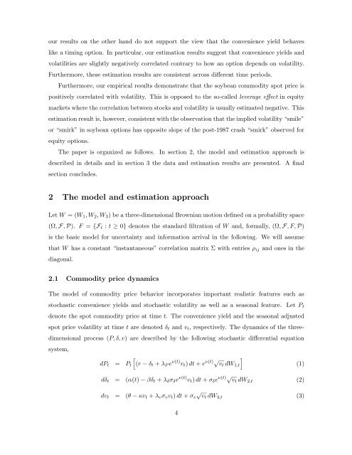
our results on the other hand do not support the view that the convenience yield behaves like a timing option. In particular, our estimation results suggest that convenience yields and volatilities are slightly negatively correlated contrary to how an option depends on volatility. Furthermore, these estimation results are consistent across different time periods. Furthermore, our empirical results demonstrate that the soybean commodity spot price is positively correlated with volatility. This is opposed to the so-called leverage effect in equity markets where the correlation between stocks and volatility is usually estimated negative. This estimation result is, however, consistent with the observation that the implied volatility “smile” or “smirk” in soybean options has opposite slope of the post-1987 crash “smirk” observed for equity options. The paper is organized as follows. In section 2, the model and estimation approach is described in details and in section 3 the data and estimation results are presented. A final section concludes. 2 The model and estimation approach Let W = (W 1 , W 2 , W 3 ) be a three-dimensional Brownian motion defined on a probability space (Ω, F, P). F = {F t : t ≥ 0} denotes the standard filtration of W and, formally, (Ω, F, F, P) is the basic model for uncertainty and information arrival in the following. We will assume that W has a constant “instantaneous” correlation matrix Σ with entries ρ ij and ones in the diagonal. 2.1 Commodity price dynamics The model of commodity price behavior incorporates important realistic features such as stochastic convenience yields and stochastic volatility as well as a seasonal feature. Let P t denote the spot commodity price at time t. The convenience yield and the seasonal adjusted spot price volatility at time t are denoted δ t and v t , respectively. The dynamics of the threedimensional process (P, δ, v) are described by the following stochastic differential equation system, dP t = P t [ (r − δ t + λ P e ν(t) v t ) dt + e ν(t)√ v t dW 1,t ] dδ t = (α(t) − βδ t + λ δ σ δ e ν(t) v t ) dt + σ δ e ν(t)√ v t dW 2,t (2) dv t = (θ − κv t + λ v σ v v t ) dt + σ v √ vt dW 3,t (3) (1) 4
where β, κ, θ, λ P , λ δ , λ v , σ δ , and σ v , as well as the correlation parameters of W , are constant parameters that we will estimate in the subsequent sections. α(t) and ν(t) are deterministic functions that aim at describing a seasonal pattern in convenience yields and volatilities; the functional forms of α(t) and ν(t) are described and discussed below. The parameters λ P , λ δ , and λ v are the risk premia on commodity price uncertainty, convenience yield uncertainty, and volatility uncertainty. We will assume markets are complete and the existence of an equivalent martingale measure, Q, so that prices on contingent claims can be uniquely derived by evaluating the relevant expectations of the discounted payoff under Q. Using a standard terminology, we will also refer to Q as the risk-neutral probability measure in the following. Under the risk-neutral probability measure, risk premia are zero and the dynamics of (P, δ, v) are described by, dP t = P t [(r − δ t ) dt + e ν(t)√ v t dW Q 1,t dδ t = (α(t) − βδ t ) dt + e ν(t) √ σ δ vt dW Q 2,t (5) √ dv t = (θ − κv t ) dt + σ v vt dW Q 3,t (6) From equations (1) and (4) it follows that the convenience yield, δ t , can be interpreted as the return shortfall on an inventory position of the specific commodity. 7 Basically, in order to break-even on the marginal inventory position, there must be a gain, or convenience yield, from holding inventory to exactly offset the return shortfall. The parameters β and κ determine the degree of reversion to the deterministic seasonal pattern in the convenience yield and the long-run volatility level θ, respectively. Likewise, σ δ and σ v are parameters that, together with the level of v t , determine the volatility of the convenience yield and the volatility of the stochastic volatility of the commodity price. The parameter r is the short default-free interest rate which is assumed constant (but we allow to vary over time in our empirical analysis). 8 The deterministic seasonal functions α(t) and ν(t) are defined as, ∑ α(t) = α 0 + (α k cos (2πkt) + αk ∗ sin (2πkt)) (7) K α k=1 7 In fact, the convenience yield may be defined as the return shortfall on holding the commodity; see, e.g., MacDonald and Siegel (1984). 8 Our pricing results will carry through if interest rates are stochastic but distributed independently of the soybean dynamics. In this case, discounting is done using the appropriate zero coupon bonds, as in our empirical approach. ] (4) 5
Page 1 and 2: Stochastic Volatility and Seasonali
Page 3 and 4: 1 Introduction This paper sets up a
Page 5: The estimated commodity price model
Page 9 and 10: Solutions to the ordinary different
Page 11 and 12: The measurement equation relates th
Page 13 and 14: and, N ˆΓ ∼ W m (N, Γ) where W
Page 15 and 16: where T s and T l refer to the rele
Page 17 and 18: prices seems lower than that of sho
Page 19 and 20: [ INSERT FIGURE 2 ABOUT HERE ] As s
Page 21 and 22: where adverse weather conditions ma
Page 23 and 24: Inverse leverage effects The correl
Page 25 and 26: (with the relevant estimated standa
Page 27 and 28: as well as changes in government po
Page 29 and 30: Besides estimating model parameters
Page 31 and 32: Chambers, M. & Bailey, R. (1996).
Page 33 and 34: Kaldor, N. (1939). “Speculation a
Page 35 and 36: Appendix Lemma 1 Let p t = log P t
Page 37 and 38: Table 2: Summary statistics for soy
Page 39 and 40: Table 4: Parameter estimates for so
Page 41 and 42: 1100.00 Futures prices in cents per
Page 43 and 44: 1.00 0.75 0.50 0.25 0.00 - 0.25 α(
Page 45: 2.00 1.50 1.00 0.50 0.00 - 0.50 α

Stochastic Volatility and Seasonality in ... - Interconti, Limited

You also want an ePaper? Increase the reach of your titles

Delete template?

Save as template?