Stochastic Volatility and Seasonality in ... - Interconti, Limited

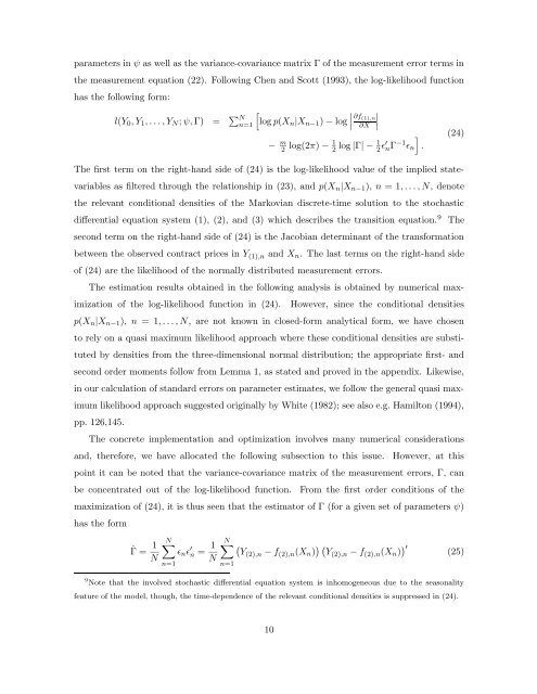
parameters in ψ as well as the variance-covariance matrix Γ of the measurement error terms in
the measurement equation (22). Following Chen and Scott (1993), the log-likelihood function
has the following form:
l(Y 0 , Y 1 , . . . , Y N ; ψ, Γ) = ∑ [
N
∣
n=1
log p(X n |X n−1 ) − log
∣
∣ ∂f (1),n
∂X
− m 2 log(2π) − 1 2 log |Γ| − 1 2 ɛ′ nΓ −1 ɛ n
]
.
The first term on the right-hand side of (24) is the log-likelihood value of the implied statevariables
as filtered through the relationship in (23), and p(X n |X n−1 ), n = 1, . . . , N, denote
the relevant conditional densities of the Markovian discrete-time solution to the stochastic
differential equation system (1), (2), and (3) which describes the transition equation. 9
second term on the right-hand side of (24) is the Jacobian determinant of the transformation
between the observed contract prices in Y (1),n and X n . The last terms on the right-hand side
of (24) are the likelihood of the normally distributed measurement errors.
The estimation results obtained in the following analysis is obtained by numerical maximization
of the log-likelihood function in (24).
(24)
The
However, since the conditional densities
p(X n |X n−1 ), n = 1, . . . , N, are not known in closed-form analytical form, we have chosen
to rely on a quasi maximum likelihood approach where these conditional densities are substituted
by densities from the three-dimensional normal distribution; the appropriate first- and
second order moments follow from Lemma 1, as stated and proved in the appendix. Likewise,
in our calculation of standard errors on parameter estimates, we follow the general quasi maximum
likelihood approach suggested originally by White (1982); see also e.g. Hamilton (1994),
pp. 126,145.
The concrete implementation and optimization involves many numerical considerations
and, therefore, we have allocated the following subsection to this issue.
However, at this
point it can be noted that the variance-covariance matrix of the measurement errors, Γ, can
be concentrated out of the log-likelihood function.
From the first order conditions of the
maximization of (24), it is thus seen that the estimator of Γ (for a given set of parameters ψ)
has the form
ˆΓ = 1 N
N∑
ɛ n ɛ ′ n = 1 N
n=1
N∑ (
Y(2),n − f (2),n (X n ) ) ( Y (2),n − f (2),n (X n ) ) ′
n=1
(25)
9 Note that the involved stochastic differential equation system is inhomogeneous due to the seasonality
feature of the model, though, the time-dependence of the relevant conditional densities is suppressed in (24).
10