Factors Affecting the Finite Element Simulation of a ROPS Test of a ...

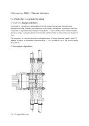
DEPARTMENT OF MANAGEMENT AND ENGINEERING
Factors Affecting the Finite Element Simulation
of a ROPS Test of a Volvo Cab
Master Thesis carried out for Volvo CE AB
at the Division of Solid Mechanics
Linköping University
January 2007
Rikard Svärd
LIU-IEI-TEK-A--07/0014--SE
Institute of Technology, Department of Management and Engineering
SE-581 83 Linköping, Sweden

Avdelning, institution
Division, Department
Div of Solid Mechanics
Dept of Management and Engineering
SE-581 83 LINKÖPING
Datum
Date
2007-01-15
i
Språk
Language
Rapporttyp
Report category
ISBN
x
Svenska/Swedish
Engelska/English
________________
x
Licentiatavhandling
Examensarbete
C-uppsats
D-uppsats
Övrig rapport
_____________
ISRN
_________________________________________________________________
Serietitel och serienummer
Title of series, numbering
LIU-IEI-TEK-A--07/0014--SE
Titel
Title
Författare
Author
Factors Affecting the Finite Element Simulation of a ROPS Test of a Volvo Cab
Rikard Svärd
Sammanfattning
Abstract
The ability to protect the operator if a rollover of a construction equipment vehicle should take
place is an essential requirement. In order to fulfil the necessities of this aspect, each cab
constructed today is provided with a Rollover Protective Structure (ROPS).
The cabs developed by Volvo Construction Equipment undergo a ROPS-test. These tests are
performed to ensure that the cab is able to uphold certain forces and consume certain energy levels
without exceeding the restrictions in terms of displacements. As a part of the design process,
Volvo uses simulations of these tests.
Comparisons made between tests and simulations have usually shown good agreements. This was
not the case in a recent comparison of results. The objective of this thesis is to explain why the
simulation of this test did not show satisfying agreement with the physical test.
By designing and constructing a welded component of standard beams and testing this as well as
developing a finite element model of the component, an investigation of the influence of different
parameters has been done.
The results from this thesis show that the major part of the divergence is due to non-correct
material data. From yield tests and hardness measurements, material data has been obtained. These
data show that the forming process, while manufacturing structural parts as well as welding these,
strengthens the material with respect to the yield strength. Another major influence on the results
comes from the modelling of welds in the FE-model.
With corrections for material data made in combination with a number of other changes of the
model, results far better than the original are obtained.
Nyckelord: finite element, simulation, material data, welding, ROPS test
Keyword

i
Abstract
The ability to protect the operator if a rollover of a construction equipment vehicle
should take place is an essential requirement. In order to fulfil the necessities of this
aspect, each cab constructed today is provided with a Rollover Protective Structure
(ROPS).
The cabs developed by Volvo Construction Equipment undergo a ROPS-test. These
tests are performed to ensure that the cab is able to uphold certain forces and consume
certain energy levels without exceeding the restrictions in terms of displacements. As
a part of the design process, Volvo uses simulations of these tests.
Comparisons made between tests and simulations have usually shown good
agreements. This was not the case in a recent comparison of results. The objective of
this thesis is to explain why the simulation of this test did not show satisfying
agreement with the physical test.
By designing and constructing a welded component of standard beams and testing this
as well as developing a finite element model of the component, an investigation of the
influence of different parameters has been done.
The results from this thesis show that the major part of the divergence is due to noncorrect
material data. From yield tests and hardness measurements, material data has
been obtained. These data show that the forming process, while manufacturing
structural parts as well as welding these, strengthens the material with respect to the
yield strength. Another major influence on the results comes from the modelling of
welds in the FE-model.
With corrections for material data made in combination with a number of other
changes of the model, results far better than the original are obtained.

iii
Sammanfattning
Förmågan att skydda föraren om en entreprenadmaskin välter är ett grundläggande
krav på fordonet. För att säkerställa uppfyllandet av detta förses hytten med en
skyddande struktur, en så kallad Rollover Protective Structure (ROPS).
De hytter som utvecklas och tillverkas av Volvo Construction Equipment genomgår
prov av denna struktur. Proverna genomförs för att säkerställa att respektive
hyttkonstruktion klarar vissa kraft- och energikrav utan att inträngningen av någon del
blir för stor i hytten. Som en del i utvecklingsarbetet genomförs finita
elementsimuleringar av dessa prover.
Prov – och beräkningsresultat har generellt uppvisat god överensstämmelse.
Bakgrunden till detta examensarbete är ett fall där avvikelserna var tämligen stora.
En struktur konstruerad av balkar av samma slag som används i hytten har provats
och detta prov har simulerats för att göra en studie av ingående finita
elementparametrar. Materialdata har tagits fram med hjälp av drag- samt hårdhetsprov.
Arbetet visar att felaktiga materialdata var en stor anledning till avvikelserna. Fler
faktorer, bland annat på vilket sätt svetsar modelleras, har en stor inverkan på
resultatet.
Med korrigeringar gjorda för materialdata och ett antal andra faktorer erhålls resultat
som är avsevärt bättre än de ursprungliga.

v
Preface
This thesis is the final assignment for graduation as a Master of Science in
Mechanical Engineering. The work has been performed at the Division of Solid
Mechanics, University of Linköping. It has been carried out for Volvo Construction
Equipment with Engineering Research as a second company with interest of the work.
I would like to thank Anders Lindkvist, M.Sc. at Volvo, Prof. Larsgunnar Nilsson at
the University of Linköping and Dr. Rikard Borg at ERAB for their help and guidance
throughout the work. I would also like to thank Mr Ulf Bengtsson, Mrs Annette
Billenius and Mr Bo Skoog at the University of Linköping for their help and support
with test preparations and performances.
Linköping, January 2007
Rikard Svärd

1
Contents
1 Introduction............................................................................................1
1.1 Background ........................................................................................................1
2 ROPS Test...............................................................................................3
2.1 Definitions...........................................................................................................3
2.2 Test Procedure ...................................................................................................3
2.2.1 Lateral loading..............................................................................................3
2.2.2 Vertical loading ............................................................................................4
2.2.3 Longitudinal loading.....................................................................................4
2.3 Test Results.........................................................................................................4
3 FE Simulation of ROPS Test ................................................................5
3.1 FE Model.............................................................................................................5
3.1.1 Geometry.......................................................................................................5
3.1.2 Boundary Conditions ....................................................................................5
3.1.3 Elements........................................................................................................6
3.1.4 Material Models............................................................................................6
3.1.5 Weld Modelling.............................................................................................6
3.2 Original Simulation Results..............................................................................7
4 Component..............................................................................................9
4.1 Choice of Component ........................................................................................9
4.2 Test Procedure and Results.............................................................................12
5 Material Testing...................................................................................15
5.1 Tensile Test.......................................................................................................15
5.1.1 Test Theory and Procedure.........................................................................15
5.1.2 Test Objects.................................................................................................17
5.1.3 Nominal Test ...............................................................................................18
5.1.4 Influence of Welding ...................................................................................19
5.2 Hardness Test...................................................................................................20
5.2.1 Test Theory and Procedure.........................................................................20
5.2.2 Test Objects.................................................................................................21
5.2.3 Nominal Test ...............................................................................................21
5.2.4 Influence of Welding ...................................................................................22
5.2.5 Influence of the Forming Process...............................................................23
6 FE Simulation of Component .............................................................25
6.1 FE Model...........................................................................................................25
6.2 Investigation of Parameters ............................................................................28
6.2.1 Number of elements.....................................................................................28
6.2.2 Element Formulation ..................................................................................28
6.2.3 Number of Integration Points .....................................................................29

6.2.4 Material Data..............................................................................................30
6.2.5 Weld Modelling...........................................................................................31
6.2.6 Heat Affected Zone......................................................................................33
6.2.7 Plastically Deformed Corners ....................................................................35
6.2.8 Combination of Heat Affected Zones and Plastically Deformed Corners..35
6.2.9 Thickness Change Update...........................................................................36
6.2.10 Globally Scaled Plastic Behaviour ...........................................................37
6.3 Analysis of Results and Final Combinations.................................................37
7 Modified Simulations of ROPS Test Performed by ERAB .............41
7.1 Material Data ...................................................................................................41
7.2 Material Data and Weld Modelling................................................................41
7.3 Material Data, Weld Modelling and Sequential Loading ............................42
8 Results ...................................................................................................45
9 Conclusions...........................................................................................47
10 Possible Future Work........................................................................49
References................................................................................................51
Appendix A: Drawings of Component..................................................53

1
1 Introduction
1.1 Background
Volvo Construction Equipment Cabs AB is located in Hallsberg. The company
develop and manufacture cabs for construction equipment vehicles. For a cab to be
approved for the use in a vehicle, a number of requirements have to be fulfilled. One
of these is that the cab has to provide the operator with proper protection in the case
of a vehicle turnover (rollover). The part of the cab structure that provides this
protection is denoted as the Rollover Protective Structure (ROPS). Each type of cab
has to be tested according to a standard that has been established by the industry. The
test is not an actual rollover but sequential quasi-static tests in a controlled manner.
These tests are simulated with the Finite Element, FE, method to obtain results as
basis for the development of the cabs. The simulations have in general shown good
agreements with the corresponding tests. In this case however, the simulation showed
results that did not agree with the corresponding test. The tests studied have been
performed by Svensk Maskinprovning AB in Malmö and the simulations were
performed by Engineering Research Nordic AB in Linköping.
1.2 Objective
The main objective of this thesis is to explain the divergent results between the tests
and the simulations performed on a ROPS. A second objective has been to exclude as
many parameters as possible from the potential reasons to erroneous results. As this
means a study of different parameters, the thesis aims at concluding the influence of
different parameters.
1.3 Procedure
The work has been divided into three main tasks. The first is to examine the models
from the simulations and the tests performed in order to find possible reasons of
divergence between the results. This has been done by comparing the geometry of the
original CAD-data with the simulation model and test geometry, a study of boundary
conditions and similar factors.
The other main task has been to create a simplified, welded structure made of
standard beams used in the cab. This component has been modelled in the same way
as the cab model and 5 test objects have been manufactured and tested. The model has
been used to determine how different parameters in the FE-model influence the results.
The third task has been to test the material used in the cab structure with respect to its
plastic behaviour. Further, a number of tests of the material properties have been
performed to estimate the size and influence of the heat affected zones at the vicinity
of the welds. The corners of the beam have been another aspect; they are plastically
formed and therefore they probably have an increased yield strength. A series of tests
has been performed to estimate this influence as well.

2
3 Simulation of ROPS Test

2 ROPS Test
2 ROPS Test
3
2.1 Definitions
ROPS (rollover protective structures)
A system of structural members whose primary purpose is to provide a seated
operator with reasonable protection in the event of a machine turnover (rollover). Non
load-carrying members as doors and windows are excluded.
DLV (deflection-limiting volume)
A volume in the cab defined by an orthogonal approximation of a large, seated
operator. No parts of the cab may penetrate this volume during the test. The size and
placement are defined in a standard description; ISO 3164:1995.
LAP (load application point)
Point on the ROPS where the test load force is applied. LAP is also the point where
the displacements are measured.
2.2 Test Procedure
To ensure that a cab manages to protect the driver in the event of a machine rollover,
tests established by the International Standards Organisation (ISO) are carried out.
The standard (ISO 3471) defines the loading of the cab as a quasi-static sequence
performed with one or more hydraulic cylinder(s). The sequence consists of three
parts; a lateral followed by a vertical and finally a longitudinal loading. In each case,
the size of the required force depends on the machine weight and no part of the
structure may intrude the DLV. When loading the ROPS in lateral direction a certain
energy level has to be reached. This amount depends on the machine mass. The rate
of deflection at the load application point shall not exceed 5 mm/s. Further, the
systems used to measure mass, force and deflection shall be capable of meeting the
requirements of another standard, ISO 9248, except that force and deflection
measurement capability shall be within + or – 5% of maximum values.
2.2.1 Lateral loading
A load distributor is used to avoid localized penetration of the ROPS structural
members. The load distributor is basically a plate and may distribute the force over a
length of maximum 80% of the ROPS length. The side loaded shall be that which
gives the most severe deflections. The initial direction of the loading shall be
horizontal and perpendicular to a vertical plane through the machine longitudinal
centreline. During the loading, deformations may cause the direction of loading to
change, which is permissible. The position of the LAP is defined on the basis of the
DLV location. The loading shall continue until the force and energy levels have been
reached. The energy is calculated as the area under the force-displacement curve
obtained at the cylinder(s).

4
3 Simulation 2 ROPS of Test ROPS Test
Figure 2.1. ROPS prior to lateral loading
2.2.2 Vertical loading
A load distributor is used in the vertical loading as well. The centre of the vertical
load shall be applied in the same vertical plane, perpendicular to the longitudinal
centreline of the ROPS, as the lateral load. The structure is loaded until the force level
specified is reached and shall support this load for 5 minutes or until any deformation
has ceased, whichever is shorter.
2.2.3 Longitudinal loading
After the vertical loading, a longitudinal load shall be applied to the ROPS. This load
shall be applied along the longitudinal centreline of the ROPS, at a load point defined
by the intersecting planes of the front and top surfaces. A load distributor may
distribute the load over a length no greater than 80% of the width. The loading is to
continue until the force level specified has been reached.
2.3 Test Results
The results from tests previously performed are presented in Figure 2.1.
Force
[kN]
300
250
200
150
100
50
0
0 60 120 180 240
Deflection [mm]
Figure 2.1. Lateral test results to the left and longitudinal test results to the right

3 Simulation of ROPS Test 5
3 FE Simulation of ROPS Test
3.1 FE Model
The FE simulations of the ROPS test have been performed by Engineering Research.
This section describes how the cab is modelled and how the simulation is performed.
3.1.1 Geometry
The geometry of the test model is taken from the original CAD data from Volvo CE.
That is, every part and its location are given from the same information as the
drawings designed for manufacturing.
3.1.2 Boundary Conditions
The ends of the circular beam that the cab rests on are constrained from all
translational and rotational movement.
Figure 3.1. The ends of the circular beam (at the arrows) are constrained from
translational and rotational movement
The load is applied by a load distributor given a prescribed motion. The load
distributor is modelled as a rigid body with the displacements perpendicular to the
loading direction constrained as well as rotations around the x-axis, see Figure 3.2. As
in the testing, the loading is defined as prescribed displacements.

6
3 Simulation of ROPS Test
Figure 3.2. The cab model with the load distributor pointed out
3.1.3 Elements
The cab is modelled mainly with four-noded shell elements of an approximate size of
10x10 mm. The element type is the fully integrated shell element type 16 in LS-
DYNA.
3.1.4 Material Models
The actual ROPS materials are modelled with a piecewise linear plasticity model.
That is, the material deforms elastically using a Young’s modulus up to the yield
strength. Thereafter, the material deforms plastically according to a piecewise linear
relation between the true stress and the true plastic strain in the plastic region.
The load distributor is modelled as a rigid body.
Some of the welds in the cab are modelled with a special material model defined
specifically for welds. This is described in the next section.
3.1.5 Weld Modelling
For the long, straight parts welded together, an automatic type of weld model may be
defined in LS-DYNA. This gives the possibilities to define a Young’s moduli,
Poisson’s ratio and a plastic behavior of the weld material as well as the possibility to
use failure criteria on the welds. By experience, failure in these tests is rare, why no

3 Simulation of ROPS Test 7
failure criterion has been used. The Young’s moduli as well as Poisson’s ratios are the
same as adjacent parts in the structure. The weld is created between nodes of each part
welded, and the weld material is used to connect them. The plastic behaviour is
ignored by defining a very high yield strength of the weld material.
In the more complex geometrical areas, constrained nodal rigid bodies are used. They
are modelled by connecting a number of nodes in each part welded, forming a rigid
body.
3.2 Original Simulation Results
The original simulation results are presented and compared to the test results in figure
3.3.
Force
[kN]
300
250
200
150
100
50
0
0 80 160 240
Deflection [mm]
Test
Simulation
Force
[kN]
200
150
100
50
0
0 80 160 240 320
Deflection [mm]
Test
Simulation
Figure 3.3. Lateral and longitudinal simulation and test results, respectively

8
4 Component

4 Component 9
4 Component
In order to evaluate different parameters and concepts of the simulation model, a sub
component was developed, manufactured and tested. The test was also simulated in
the finite element program LS-DYNA with different sets of design parameters.
4.1 Choice of Component
The idea has been to test a common structural component of the cab – two beams
welded orthogonally to each other. The beams are standard thin-walled beams, with a
square profile, also used as B-pillars in the cab. The original idea of geometry was a
closed structure of four beams. Hand calculation showed that the test machine we had
access to did not have the load capacity enough why the geometry in Figure 4.1 was
proposed.
Figure 4.1. Component geometry
In order to verify that the test machine most probably would manage to plastically
deform the structure, the following check was done.
Using the theorem of rigid plasticity and the upper bound theorem, a limit analysis
may be done according to Odenö and Klarbring (1984). That is, an assumption is
made that the cross section of a beam is fully plasticised when the moment acting on
the beam corresponds to the stress in the entire cross section to be equal the yield limit
of the material. When this moment is reached, the structure cannot carry any more
load but will collapse.

10
4 Component
In this case, the cross sections of the beams are quadratic with the width 80 mm and
thickness 6 mm (the radius of the corners are neglected, i.e. in this case a conservative
assumption).
t
y
x
b
b
Figure 4.2. Simplified cross section of the beams
With side length b and thickness t according to Figure 4.2 the moment around the x-
axis may be calculated using the yield limit σ of the material
Where
M
fp
= 2σ
Ybt
(4.1a)
2
1 b
M
fp
= 2σ
Ybt
(4.1b)
4
2 b
1
M
fp
is the moment required to plasticise the lower and upper parts of the
2
beam in Figure 4.2 and M
fp
the moment required to plasticise the sides of the beam.
The index fp means fully plastic.
1
2
M
fp
and M
fp
may now be added to a total moment M
fp
needed to plasticise the
entire cross section
Y
M
fp
3b
2 t
= σ
Y
(4.2)
2
The test object is to be loaded in compression in the horizontal direction according to
the orientation of the left part of Figure 4.1. Referring to Odenö and Klarbring (1984),
a collapse load calculated for an assumed collapse mechanism is equal to or greater
than the true collapse load.
The assumption made here is that one plastic hinge is enough to collapse the structure
according to Figure 4.3.

4 Component 11
L
P
θ
P acm
δ
2
L
P acm
P
Plastic hinge
Figure 4.3. One plastic hinge at the joint is the assumed collapse
mechanism (acm) which gives the change in angle θ for each
beam and a total deflection δ. The beams have the length L and a
force P is applied on the structure
The supplied power is equal to the dissipated power which gives the relation
acm
P δ = 2M θ
(4.3)
fp
Where the dot above δ and θ indicates the time derivative of each variable. If δ is
assumed small, the angle θ is also small and the simplification stated in Equation (4)
may be done using the length L
δ = L sin θ = Lθ
(4.4)
The equations (2), (3) and (4) may now be combined to the following expression.
P
acm
2
2M
fp 3b
t
= = σ
Y
(4.5)
L L
The yield strength of the material is 355 MPa according to the material supplier. Due
to the size of the test machine, the maximum allowable lengths of the beams are 452
mm on the inside of the component. By adding half the width of the beams, the length
used for this calculation becomes 492 mm.
This gives numerically that the force needed according to the assumed collapse
mechanism is
2
acm 3⋅80
⋅ 6
P = ⋅355
= 83.1kN (4.6)
492
This is permissible since the maximum capacity of the test machine is approximately
100 kN.

12
4 Component
The geometry was settled according to Figure 4.4 and the component was
manufactured at Volvo CE.
Figure 4.4. One of the five test components
Drawings of the component are presented in Appendix A.
4.2 Test Procedure and Results
The tests were carried out at the University of Linköping in an INSTRON 5582 test
machine. The test object was mounted in the machine as presented by Figure 4.5. The
machine has a maximum force of 100 kN and the ability to deliver this force a
distance corresponding to the length of the test objects. During the test performance
the load cell included in the machine registered the force at the same time as the
displacement was recorded. The software Bluehill was used to control the test and
extract test results, which were defined as curves where the force is plotted as
function of the displacement. The tests were carried out with a loading rate 5 mm/min,
which certainly is to be considered as a static loading.
Figure 4.5. Component in test machine before loading

4 Component 13
Figure 4.6. Component after test
Force (kN)
70
60
50
40
30
20
10
0
0 100 200 300 400
Displacement (mm)
Test 1
Test 2
Test 3
Test 4
Test 5
Figure 4.7. Test results of the component
As seen in Figure 4.7, the results from the component tests are homogeneous, with
one small exception; test object 5 showed somewhat lower force level throughout the
test. The first three tests were performed to a displacement of 200 mm and the last
two tests to a displacement of 300 mm. Even though the results are more or less the
same for the five tests, they are not totally identical. Test 2 is established as a
representative result, why this is the case chosen for comparisons with the FE results
in the following.

14
5 Material Testing

5 Material Testing
15
5 Material Testing
Correct material data is of great importance while striving for correct FE simulation
results. The nominal yield strength of the material according to the supplier is greater
than 355 MPa. Because of the uncertain mechanical properties of the beams used in
the cab and the tested component, various mechanical tests have been made. The test
procedures and results are presented in this section.
5.1 Tensile Test
5.1.1 Test Theory and Procedure
When a tensile test is performed, the measured quantities are the loading force and the
displacement. The displacement is primarily measured with an extensometer as the
current length L of the test length. The initial length L
0
in this case was 50 mm. The
machine used was an INSTRON 5582. This machine is an electromechanical test
machine, which in this case was controlled by the software Bluehill. The load cell of
the machine measures the force.
The yield tests have been performed as described in the Swedish Standards Institutes
document SS-EN 10002-1 (2001). This standard describes in details the test
parameters such as the geometry of the test specimens and the maximum strain rate
during loading. The geometry in Figure 5.1 presents some rather peculiar dimensions.
This is due to the directives in the standard used, which defines certain relations, such
as a dependency between the cross sectional area and the initial length.
Figure 5.1. Geometry properties of the tensile test specimen
According to the standard, the speed of the test may not exceed 0.86 mm/min why a
speed of 0.8 mm/min was used. Due to concerns of the test equipment, the yield tests
were terminated at a strain of about 20%.
In order to evaluate the measured quantities and further on derive curves to use as
input to LS-DYNA, the following expressions are useful.

16
5 Material Testing
The force F gives, divided by the original area Dahlberg (2001):
F
σ (5.1)
E
=
A 0
Where σ
E
is the engineering stress.
The current length L gives, together with the initial length L 0
:
L − L
0
ε
E
=
(5.2)
L0
Where ε
E
is defined as the engineering strain.
The true stress σ
T
may now be defined as
F
σ
T
=
(5.3)
A
where A is the current cross-section area of the test specimen.
The true, or logarithmic, strain ε
T
for large deformations is Dahlberg (2001)
⎛ L ⎞
ε =
⎟
⎜
T
ln (5.4)
⎝ L
0 ⎠
With the assumption that plastic deformation does not change the volume of the test
specimen, the following expression may be used:
A reformulation of Equation (2) gives:
A
0
L0
= AL
(5.5)
L
L
0
ε + 1
(5.6)
= E
Equation (6) in Equation (4) gives
ε ln( ε +1)
(5.7)
T
=
E
Equation (1) and (3) may be combined to
A
= σ
E
(5.8)
A
σ
0
T
A combination of Equation (5) and (6) leads to

5 Material Testing
17
A
0
A
L
L
=
E
0
= ε + 1 (5.9)
This may be used in Equation (8) to establish the expression
σ σ ( ε +1)
(5.10)
T
=
E E
The equations above allow determination of the true strain and the true stress from
the measured quantities and apply for strains below localization.
The engineering strain may be divided into one elastic part
, i.e.
pl
ε
E
el
ε
E
and one plastic part
ε = ε + ε
(5.11)
E
el
E
Using Equation (11) and the following expression Dahlberg (2001)
el σ
E
ε
E
= (5.12)
E
where E is Young’s modulus, give
pl
E
ε
pl
E
σ
E
= ε
E
−
(5.13)
E
Equation (13) may finally be combined with Equation (7) as
pl σ
E
ε
T
= ln( ε
E
− +1) (5.14)
E
The results obtained from testing and calculated with Equations (10) and (14) will
later be used as material data input in LS-DYNA.
5.1.2 Test Objects
The test objects are milled out from an extra component made for this purpose. All
machining were performed with controlled cooling to minimise heat effects. The
specimens are specified with respect to geometry in the previous section and further
details are defined in the corresponding following sections.
None of the specimens were perfectly flat after being milled out. This implies the
presence of rather large residual stresses. In total, seven test specimens were made
and the extensometer was mounted on the convex and concave side every other time,
respectively. No significant differences in the results were observed why no further
notice was taken on this matter.

18
5 Material Testing
5.1.3 Nominal Test
The tests defined as nominal are milled out from the middle of a beam flange, Figure
5.3.
Figure 5.3. Test specimens before milled out of the beam
Figure 5.4. Test specimens D1 and D2. The upper D1 after testing
and the lower D2 before testing
Five test specimens were milled out of the beams and tested. The test results are
presented in Figure 5.5.

5 Material Testing
19
600
Engineering stress (MPa)
500
400
300
200
Test 1
Test 2
Test 3
Test 4
Test 5
100
Figure 5.5. Nominal yield test results
The results from the specimens are quite equal, especially concerning the yield
strength. The yield strength was found to be 415 MPa, significantly higher than the
nominal 355 MPa guaranteed by the supplier.
5.1.4 Influence of Welding
0
0 5 10 15 20 25
Engineering strain (%)
The beam profiles are longitudinally welded along one of the flanges. In order to
examine the influence of the longitudinal weld and later on study the relation between
hardness and yield strength, two tests containing this weld were performed. The weld
is completely flat on the outside of the beam but the weld material on the inside were
milled away in order to grip the test specimens properly.
Figure 5.6. Test specimen containing a weld. The weld is milled
at the wider areas at the end in order to grip the specimen properly

20
5 Material Testing
800
700
600
500
400
300
200
100
Figure 5.7. Tensile test results from the welded areas of a beam profile
The yield strength is approximately 50 % higher in the welded areas at the same time
as the ductility is a lot lower. The welded area fracture at about 10 % strain while the
nominal tests were stopped at about 20 % strain.
5.2 Hardness Test
Engineering stress (MPa)
0
0 2 4 6 8 10 12
5.2.1 Test Theory and Procedure
Engineering strain (%)
Test 6
Test 7
According to Davis et al. (1998) and the course file in Experimental Evaluation of
Fatigue and Fracture, there are a linear relationship between the Vickers hardness and
the yield strength of the kind of material used. The Vickers hardness of a material is
measured by pressing a diamond into the test specimen. The diamond is a grinded
pyramid with a top angel of 136˚, which gives two diagonals when pushed into the
test specimen. The value of the Vickers hardness is then obtained from the mean
value of these diagonals whose Vickers hardness Hv is derived according to
136
2F
sin( )
Hv =
2
(5.15)
2
d
where F is the test force in kp and 1 kp = 9,80665 N.
d is the mean of the diagonal length in mm.
Equation (15) may be simplified to
see Peng et al. (2005).
1,854F
Hv = (5.16)
2
d
Before a test may be done, the test specimen has to be prepared by grinding. This is
done to avoid rough surfaces which may give false results, e.g. due to the diamond
hitting a top of the rough surface which would give a too small hardness value. The

5 Material Testing
21
preparation grinding is performed in 5 steps; by grinding with silicon papers of 220,
500, 1200, 2000 and 4000 grains per mm 2 respectively. For smaller objects (in this
case the corners and the nominal test specimens) it is convenient to cast the specimen
into a polymer material in order to fix and orient the test as desired before grinding.
Figure 5.8. A test specimen in the hardness tester
The tests were carried out in a hardness tester called LECO M-400. This machine is
basically a microscope with an indenter which may be loaded with a range of masses.
The maximum mass 1 kg was chosen because of the higher accuracy that comes with
a larger mass. The loading was held constant during 10 seconds before the diamond
was removed. Next step was that the optical instrument was put in place to make a
photo of the impression. The magnification used was 55x. The photo was then
imported to the image analysis software called microGOP 2000/S. The four corners
were marked on the screen, on which the program responds with a Vickers hardness
value.
5.2.2 Test Objects
The aim of the hardness tests is to evaluate the changes in the material due to welding
and the plastic deformation of the beams. The beams are roll formed and the data
given by the material supplier is valid for plane sheets, i.e. not taking any cold
forming into account. The test objects are therefore chosen as follows: In total five
pieces for testing the welding and heat affected zones. Three pieces for testing the
corners of a beam and three nominal test pieces picked in the middle of a beam.
The test objects for hardness measures were taken from the same component as the
tension test objects and were milled out of the beams.
5.2.3 Nominal Test
To have a reference value for comparison of values from the heat affected zones and
welds as well as the corners, a series of nominal tests were carried out. The three test
objects showed uniform results from the test series carried out. In total, 18
measurements were performed and the result is presented in Table 5.1.
173,2 174,21 172,53 173,49 171,23 173,18
174,19 171,89 171,61 173,66 175,08 175,46
177,9 172,2 176,87 174,5 172,85 169,54
Table 5.1. Results from nominal hardness tests
The mean value was determined to be Hv=173,8 N/mm 2 .

22
5 Material Testing
5.2.4 Influence of Welding
Two different kinds of welds are present in the structure. The first (1) is present in
each beam; the beams are made from sheets that are roll formed to the desired shape
and welded along the whole length. The other kind of weld (2) is the one that joins the
beams together.
2
1
Figure 5.9. Two types of welds
The test specimens used were machined (milled) from the beams according to Figure
5.10.
The measurements of the first type of weld were made in the area corresponding to
the tensile test specimens. Two test specimens were milled out of one of the beams
and the hardness were measured across the pieces. The average of the two specimens
were obtained as Hv = 231,5 N/mm 2 and Hv = 220,3 N/mm 2 , respectively. This gives
an average of both test specimens of Hv = 225,9 N/mm 2 .
The linear relation between the Vickers hardness and the yield strength may now be
verified. The yield strength of the test specimen milled out in the centre of the weld
were determined to 537 MPa. The nominal test specimens gave a yield limit of 415
537 =1,29. The corresponding quotient of the Vickers
MPa which gives the quotient 415
225 ,9
hardness is = 1,30. That is, a linear relation between the Vickers hardness and
173,8
yield limit of the material is verified. The linear relation is proposed by Davis et al.
(1984) and Peng et al. (2005).
The second type of weld tested is the weld that joins the two beams together. The test
specimens were milled out according to Figure 5.10.

5 Material Testing
23
Figure 5.10. The locations of the test specimens and the grinded results
As presented in Figure 5.10, three test specimens were milled out and tested. The
hardness measurements started in the middle of the weld and were then performed
with a distance of 2 mm between each measurement along the specimen direction
from the weld. The test results are presented in Figure 5.11.
Vickers
hardness
(N/mm2)
215
210
205
200
195
190
185
180
175
170
0 10 20 30 40 50
Position (mm)
Figure 5.11. The Vickers hardness as function of distance from the centre of
the weld. The dotted curve is a mean from three tests and the line a
linearisation of the mean
5.2.5 Influence of the Forming Process
The material data provided by the material supplier is valid for a steel sheet before
roll forming and welding. Due to the fact that the corners are plastically deformed, the
material probably undergoes a change of behaviour. Therefore, tests have been
performed to estimate this change.
The Vickers hardness were measured along the corners, Figure 5.11.

24
5 Material Testing
Position 0
Figure 5.11. A corner test specimen in its polymer fixture. Position 0
defines the starting position of the measurements
220
215
210
205
200
195
190
185
180
Vickers hardness
(N/mm2)
0 5 10 15 20 25 30 35 40
Position (mm)
Figure 5.12. Vickers hardness as function of position. The start position is
defined in Figure 5.11. The arrows points out the start, centre and end of the
curvature at the corner, respectively. The dotted curve represents a mean value
of the three test specimens and the smooth curve is a fifth order representation
of the mean
By using the linear relation between Vickers hardness and yield strength combined
215
with yield test data, the maximum yield strength in the corner is 415 = 513 MPa.
174

6 FE Simulation of Component 25
6 FE Simulation of Component
6.1 FE Model
The geometric model for the simulations was created in the pre-processor TrueGrid,
XYZ Scientific Applications, Inc (2001). That is, the different parts were modelled
and divided into discrete elements in the latter software. The model was then
transferred to the pre-and postprocessor LS-PrePost to complete the model with
respect to material models, boundary conditions etc.
The basic model was made to be as comparable as possible to the cab model. The
element size is similar, i.e. approximately 10x10 mm, the material parameters are
similar, etc. A summation of the basic model follows.
Figure 6.1. The basic model for FE simulations
The model includes the same parts as the tested component. In addition, two parts are
added in order to define the boundary conditions. The lowermost part in Figure 6.1 is
a rigid body which is constrained with respect to all translations and all rotations. A
contact is defined between this part and the lower force plate of the actual component.
The uppermost part is rigid also and all rotations are constrained. The difference from
the lowermost part is the translation; the uppermost part is given a prescribed
displacement downwards in Figure 6.1. In order to avoid peaks of reaction forces and
dynamic responses, the curve defining the motion smoothes the displacement in the
beginning of the loading, see Figure 6.2. Furthermore, this gives a better chance to
correctly treat the contacts.

26
6 FE Simulation of Component
Prescribed velocity (m/s)
2
1,6
1,2
0,8
0,4
0
0 0,05 0,1 0,15
Time (s)
Figure 6.2. The prescribed displacement of the uppermost part in the FE
model
The velocity of the uppermost part is high compared to the velocity used for testing
the component. The high velocity is chosen to save computing time and could involve
dynamic influences on the results. In order to check this, the level of kinetic energy is
compared to the total energy throughout a simulation, Figure 6.3.
8
Energy (MJ)
6
4
Total energy
Kinetic energy
2
0
0 0,05 0,1 0,15
Time (s)
Figure 6.3. Total and kinetic energy vs. time. The kinetic energy is
close to zero
The responses of the simulations do include oscillations. The response has been
filtered in all result diagrams with an SAE filter at the threshold frequency 60 Hz.

6 FE Simulation of Component 27
50
45
40
35
30
25
20
15
10
5
0
Force (kN)
Original
Filtered
0 50 100 150 200 250
Displacement (mm)
Figure 6.4 The effect of filtering, results from the basic model
The component is built up by five parts; two beams and three metal sheet parts. The
parts are welded together and in the basic model this is modelled with constrained
nodal rigid bodies (CNRB`s). The most of these connections are defined by one node
in each of the two parts joined by the weld and represents a rigid body that connects
them.
Figure 6.5. Example of nodal rigid bodies
The deformations of the FE model were in all models very much like the
deformations in the tested component, Figure 6.6.
Figure 6.6. The deformed component to the left and the corresponding
deformed FE model to the right

28
6 FE Simulation of Component
6.2 Investigation of Parameters
6.2.1 Number of elements
Two different models have been examined with respect to the number of elements, or
element size. The first size was the same as in the cab model; approximately 10x10
mm. This gave a total of 3184 shell elements, which are used to model the component.
The second size meant that each element length where divided into two, giving an
element size 1/4 of the original and a total of 12736 shell elements.
Force (kN)
45
40
35
n elements
30
25
4xn
20
elements
15
10
5
0
0 50 100 150 200 250
Displacement (mm)
Figure 6.7. Influence of the element size. The n element curve is the
uppermost.
As shown, the increase in the number of elements lowers the force response. By using
smaller elements, more degrees of freedom are used. This gives a less stiff component
with a larger displacement at the same load level.
6.2.2 Element Formulation
The default element formulation in LS-DYNA is the Belytschko-Lin-Tsay element
(type 2). In the original cab model, however, fully integrated shell element type 16 is
used. Element formulation 16 gives a more correct result. Element formulation 2 is
default due to the efficiency of the elements; they save computing time with an
acceptable accuracy. Figure 6.8 presents the differences in response between the two
element types.

6 FE Simulation of Component 29
70
Force (kN)
60
50
40
30
20
Test
Type 16
Type 2
10
0
0 50 100 150 200 250
Displacement (mm)
Figure 6.8. Influence of element type. The internal positions of the curves are
the same as the indices
The type 16 element used in the cab model is stiffer than type 2 element since it better
approximates the stress field. Type 16 is more accurate, but also more timeconsuming.
6.2.3 Number of Integration Points
Shell elements are basically defined in one plane only. A thickness of each shell is
defined, but there is no stress in the thickness direction. Through this plane a number
of integration points are defined in which the stresses and strains are evaluated
through the simulation. Basically, it is a choice between accuracy (the more
integration points, the better result) and time (the more integration points, the longer
the computing time). Defaults in LS-DYNA are three integration points for crash
analysis, five points for metal forming and seven points for spring back analysis. Five
points are however often used in this kind of simulations in order to get one point in
the middle of the thickness and better accuracy due to more points than the default
three.
As mentioned, five integration points are used in the cab model and therefore the first
choice and also used in the reference case. Three different numbers of integration
points have been used to evaluate the influence of this parameter; 2, 5 and 9 points,
respectively.
Force (kN)
70
60
50
40
30
20
10
Test
NIP=5
NIP=2
NIP=9
0
0 50 100 150 200 250
Displacement (mm)
Figure 6.9. The (non-existing) influence of number of integration points (NIP)

30
6 FE Simulation of Component
The number of integration points does not influence the response in any significant
way. The reason for this may be that the most of the structure is loaded in pure
bending while the flange thickness is small compared to the width of the beams. This
gives more or less constant stresses through the flange thickness.
6.2.4 Material Data
The material parameters defined in the FE model are density, Young´s modulus,
Poisson’s ratio and a curve defining the yield stress and relationship between true
stress and true plastic strain, see Figure 6.10.
In all analyses presented in this section, Young’s modulus E = 200 GPa, Poisson’s
ratio μ = 0.3 and the density ρ = 7800 kg/m 3 have been used. The parameter changed
and compared in this section is the curve describing the relation between true plastic
strain and the yield stress.
The original cab model had a curve defining this relation for the material of the B-
pillars with a yield strength of 275 MPa. An early statement in this work was that this
curve probably was a bad representation of the material, which according to the
supplier has a yield strength of at least 355 MPa. Therefore, the curve was scaled with
a factor 1.33 which gave a yield strength of 367 MPa. The tests of the material from a
beam presented in Section 5 gave a yield limit of 415 MPa. The data from testing
were reformulated to be a relationship between true plastic strain and true stress as
derived in Chapter 5. Since the tests were terminated when the strain was about 20 %,
the curve was extrapolated with a power law function, Figure 6.10.
True stress
(MPa)
900
800
700
Test data
600
Power law
500
400
300
200
100
0
0 0,2 0,4 0,6 0,8 1 1,2
True plastic strain (-)
Figure 6.10. The test data in the thicker curve reaches a strain of approx. 0.2.
The power law curve is used as extrapolation of the curve to the strain 1.0

6 FE Simulation of Component 31
900
800
700
600
500
400
300
200
100
True stress
(MPa)
Test data
Original data scaled
(factor 1.33)
Original material
data
0
0 0,2 0,4 0,6 0,8 1 1,2
True plastic strain (-)
Figure 6.11. Different plastic hardening curves. The original yield strength is
275 MPa, the scaled 367 MPa and the yield strength from tests is 415 MPa.
The internal positions of the curves are the same as the indices
The results from FE simulations with the three curves above used as input along with
test results are presented in Figure 6.12.
Force (kN)
70
60
50
40
30
20
10
0
0 50 100 150 200 250
Displacement (mm)
Test
415 MPa
367 MPa
275 MPa
Figure 6.12. Response of different plastic hardening curves compared to
test results. The internal positions of the curves are the same as the indices
Figure 6.12 presents the results from testing, simulation with nominal strength test
data, simulation with the material yield strength 367 MPa and lowermost 275 MPa,
respectively. The material data with yield limit 367 MPa has been used throughout the
series due to the likeliness of being a correct strength before material tests were
carried out. This was not, however, corresponding to the true value presented by the
graph “415 MPa”, obtained from tests. These results will be further discussed later.
6.2.5 Weld Modelling
Three main methods of modelling the welds have been examined. The first is the
same as in the cab model; constrained nodal rigid bodies. In this case, two or more
nodes are defined as a nodal rigid body with the displacements prescribed to be the
same in all included nodes. The second method of modelling the welds is using

32
6 FE Simulation of Component
4-noded elements and in the third method the welds are modelled using 3-noded
elements. In these cases, the material modelling of the weld part is the same as for the
beams. As the welds seem stiff when studying actual test structures, a case with a
rigid material model applied to 4-noded shell elements has been examined as well.
The three different weld-modelling methods are presented graphically in Figure 6.13
and 6.14. The results of the weld modelling aspects are presented in Figure 6.15.
Figure 6.13. From the left: CNRB, 4-noded and 3-noded shell modelling of the
weld. The 3-noded model is actually a combination of 3- and 4-noded shell
elements
Figure 6.14. Model with short CNRB´s
Force (kN)
70
60
50
40
30
20
10
Test
Rigid 4-
node
3-node
4-node
CNRB
Short
CNRB
0
0 50 100 150 200 250
Displacement (mm)
Figure 6.15. Influence of different methods of weld modeling. The internal
positions of the curves are the same as the indices
From the top in Figure 6.15 the results from the test are followed by the results from a
model with rigid 4-noded elements used for weld modelling. The third from the top is
a model with 3-noded elements and the fourth is a model with 4-noded elements with

6 FE Simulation of Component 33
the same material data as the beams. The second lowermost curve is from a model
with constrained nodal rigid bodies (CNRB´s) for weld modelling. In this case, the
length of the CNRB´s corresponds to the length of the weld in the physical structure.
The lowermost curve represents the results of where CNRB´s with the shortest
possible lengths are used for weld modelling.
The results points out the importance of modelling the welds with a correct geometry.
CNRB´s may be used with results reasonable accuracy as long as the length of the
rigid bodies are correct.
The results from the rigid 4-noded shell element weld model may seem as the best
choice. Later simulations including correct material data show however that this type
of model is over-stiff.
6.2.6 Heat Affected Zone
In order to model the influence of the heat affected zones near the weld that connects
the two beams, the parts may be divided into sub parts. The concept is to divide one
beam into several parts in order to give different areas of the beam dissimilar material
behaviour. To split up a beam, the results from the testing in Section 5.2.4 are used.
Basically, three different zones are defined, as presented in Figure 6.16.
Zone 1
Zone 2
Zone 3
Figure 6.16 The different zones around the weld
Zone 1, in the middle of the weld, has a plastic behaviour of the material scaled with
the factor 1.19. This value is obtained by dividing the Vickers hardness of the material
in the weld with the nominal Vickers hardness (in this case 207/174=1.19, Chapter 5
presents the details). Zone 2 is given the factor 1.15 and zone 3 the factor 1.10. Figure
6.17 presents the meaning of this graphically and the result is presented in Figure 6.18.

34
6 FE Simulation of Component
900
800
700
600
500
400
300
200
100
0
True stress
(Mpa)
Factor 1.20
Factor 1.15
Factor 1.10
Original
0 0,2 0,4 0,6 0,8 1 1,2
True plastic strain (-)
Figure 6.17. The use of scale factors due to heat affected zones.
The different curves are used in the part of the beam corresponding
to each hardness value
To scale the entire plastic behaviour is a generalisation made from the increased yield
strength.
70
60
Force (kN)
50
40
30
Test
Scaled zones
Original
20
10
0
0 50 100 150 200 250
Displacement (mm)
Figure 6.18. Influence of the heat affected zones. The internal positions of the
curves are the same as the indices
Figure 6.18 shows the influence of the heat affected zones. Note that the basic
material data still has the yield strength 367 MPa, giving the possibility to compare
the original data to the case were the heat affected zones have been scaled according
to hardness tests performed.
The influence from the heat affected zones is important and gives a response much
stiffer than the original. A great deal of the plastic deformation is located in the heat
affected areas.

6 FE Simulation of Component 35
6.2.7 Plastically Deformed Corners
As previously described, the corners of the beams are plastically deformed during the
manufacturing process. The different hardness values due to this phenomenon are
presented in Section 5.2.5 and the different zones with their scale factors for plastic
behaviour are presented in Figure 6.19
Zone 2a
Zone 1
Zone 2b
Figure 6.19. The different zones in the strain hardened corner
70
Force (kN)
60
50
40
30
20
Test
Scaled corners
Original
10
0
0 50 100 150 200 250
Displacement (mm)
Figure 6.20. Influence of the plastically deformed corners
The influence of the strain-hardened corners is not as significant as that from the heat
affected zones, probably because the corners outside the heat affected zones are not
much plastically deformed.
6.2.8 Combination of Heat Affected Zones and Plastically Deformed
Corners
This model is, as stated above, a combination of the modelling of heat affected zones
and plastically deformed corners described in the two previous sections.

36
6 FE Simulation of Component
70
Force (kN)
60
50
40
30
Test
Heat+corners
Original
20
10
0
0 50 100 150 200 250
Displacement (mm)
Figure 6.21. The results of modelling the heat affected zones and
plastically deformed corners in the same model. The internal positions of the
curves are the same as the indices
The results of heat affected zones in combination with the strain-hardened corners are
not much different from that of the heat affected zones only, see previous comments.
6.2.9 Thickness Change Update
By default, no thickness updates due to membrane straining are made. That is, even if
an element is heavily deformed, the thickness remains constant as defined in the input
data. A simulation with thickness update due to plastic strains has been performed and
the result is presented in Figure 6.22.
70
Force (kN)
60
50
40
30
20
Test
Thickness update
Original
10
0
0 50 100 150 200 250
Displacement (mm)
Figure 6.22. Influence of thickness update due to plastic strains
The influence of the thickness update is not significant in the area of the greatest
interest, which may be defined as the left area of Figure 6.22. It is, as expected, more
significant when the plastic deformations are large, to the right in the graph.

6 FE Simulation of Component 37
6.2.10 Globally Scaled Plastic Behaviour
The sections 6.2.6 and 6.2.7 describe the influence of the raised yield strength due to
previous heating and plastic deformations of the beams. The aim of the simulation
presented in this section is to present a factor to use for scaling the material curve to
let the whole model share one material. The material data scaled are the results from
tensile tests. The curve in the figure below therefore represents a combination of two
models from sections 6.2.4 and 6.2.8 including a weighted, global scale factor.
If the corners influenced by plastic deformation and the areas influenced by heat near
the welds are weighted relative the total amount of material, a scale factor of 1.08 is
obtained. The heat affected part of the material at the joint between the welds
however represents a major part of the material that plastically deforms in the
simulation. Therefore, a 50 % increase of the factor 1.08 was assumed to represent the
larger influence. This gives a factor of 1.12.
70
Force (kN)
60
50
40
30
20
Test
Scaled
material
Original
10
0
0 50 100 150 200 250
Displacement (mm)
Figure 6.23. Influence of a global scale factor of 1.12 for the
plastic behavior of the material. The internal positions of the curves are the
same as the indices
The globally scaled material gives a response that is greatly improved. It is, however,
hard to know the correct scale factor to use in different loadings and structures. The
factor approximated in this case gives good results, but it is not generally applicable.
6.3 Analysis of Results and Final Combinations
A number of simulations have been carried out using different combinations of the
parameters. Only the basic influences of some parameters have been presented in the
previous sections.
That a decrease of element size gives a weaker response is natural. The displacements
of an element are defined in the nodes which mean that a larger element gives a

38
6 FE Simulation of Component
reduced number of degrees of freedom. This is always a balance act between accuracy
and computing time needed for an analysis.
The element formulations investigated gave slightly different results due to different
approximations of the stress field. As in the case of element size, this is as well a
choice between accuracy and speed; element formulation 16 is more accurate but in
this case about three times more computing time consuming. The element used in all
other cases, however, is element type 16 because of its performance combined with
the ability to compare different results.
Regarding the number of integration points, there are no significant differences
between the three cases examined - 2, 5 and 9 integration points. This could be
explained by the geometric characteristics of the structure. The thickness of a beam
flange is small compared to the widths which may give a behaviour that is close to
constant through the flange thickness. Five integration points are used in all other
cases in order to obtain comparable results.
The material data is decisively the most important factor of success in the striving for
correct results. It is probably also the most extensive field of the parameters
examined. The material data used in the original cab model had a yield limit of 275
MPa, and was at an early state assumed to be incorrect. This was proved to be a
correct assumption later on by testing the material; the yield strength of a beam is 415
MPa and depends on the location in the beam.
No non-isotropic behaviour has been studied, which is one of the major assumptions
used to describe the material. This could be justified by the loading of the structure,
which gives a bending of the beams with loading in the longitudinal direction. The
deformation in the buckling zone near the weld between the beams is however
complex and possibly not negligible in the transverse direction. Despite this, the unisotropic
behaviour has not been further studied. The fact that the material data is nonhomogeneous
within the parts makes it even more complex to model. If corrections
are made for the known diversities of plastic behaviour, good results are achievable.
The attempt of scaling the whole model to a mean level with respect to yield strength
succeeded with respect to obtaining results that coincides with test results from the
component in this report. It is however hard to draw any general conclusions. It might
not be a good factor in another loading case or structure.
The weld modelling comparisons show a large influence of the weld modelling. All
models give reasonable responses for the elastic part of the compression. This is not
enough; a correct behaviour is demanded in the plastic regime as well. The
comparisons made show that a model with rigid shell elements gives a too large
stiffness of the structure. When comparing the other cases, the most important factor
seems to be to model the weld with a length corresponding to the reality. That is, the
size (length) of the weld model should be the same as the actual weld. If this is done
and combined with correct material data, the maximum load will be correct, see
Figure 6.24.

6 FE Simulation of Component 39
In order to describe the plastic behaviour throughout the simulation correctly, the 3-
noded shell element representation gives satisfying results. This model is the one with
the most realistic representation of the weld material.
No statistical studies have been performed, which makes the combination of different
combinations of parameters somewhat hazardous. Errors may still be included in the
result but cancelled out by each other. The most correct modelling aspects however
ought to be a combination of small elements, material data from tensile tests and
hardness tests combined with 3-noded shell elements for the weld modelling and
element formulation 16. The results of this combination prove the validity of the
investigation performed, Figure 6.24.
Force (kN)
70
60
50
40
30
20
Test 2
FE
10
0
0 50 100 150 200 250
Displacement (mm)
Figure 6.24. The most correct combinations of parameters give good results.
The most important parameters in this context are material data according to
yield- and hardness tests and 3-noded shell elements with a size corresponding
to reality
The results above are satisfying with respect to correctness. Despite this, the
parameters used are not that good in means of implementation in a cab model. That
would be very time-consuming due to a great deal of manual work as well as a
computing time needed for the analysis in the order of eight times longer than the
original.
The combination of factors to use in the cab model is not utterly obvious, but a
suggestion of modelling aspects are to use the original size of elements combined
with somewhat scaled yield test data; for example a factor of 1.10 might be used. The
lowered factor 1.10 instead of the previously used 1.12 is suggested because of the
deformation modes. In the tested component a great part of plastic deformations are
found in the heat affected zone. In the cab, deformations are more spread along the
beams and the beams are generally longer than the one used in the component.
Further, it is important to study the welds of the cab with respect to geometry –
constrained nodal rigid bodies may be used as long as the lengths of the welds are
represented properly.

40
6 FE Simulation of Component
The combination suggested above gives component model results according to Figure
6.25.
70
Force (kN)
60
50
40
30
20
Test
FE,
proposed
model
FE, original
10
0
0 50 100 150 200 250
Displacement (mm)
Figure 6.25. Results obtained with the proposed setup of parameters
compared to test results and the original FE results. The internal positions of
the curves are the same as the indices
The proposed set of parameters is based on globally scaled material properties with
the factor 1.10 and CNRB´s with lengths corresponding to the length of the physical
weld. It gives reasonable accuracy without extending the computational work too
much.

7 Modified Simulations of ROPS Test Performed by ERAB 41
7 Modified Simulations of ROPS Test Performed by ERAB
Three main changes have been done in the cab model. These are change of material
properties, changes in geometry/weld modelling and the implementation of a
sequential loading, respectively. The different changes and their influence on the
results are presented in this section. All results presented are from longitudinal
loading which had the largest errors in the original simulation. All simulations of the
cab model have been performed by ERAB.
7.1 Material Data
In the original model, the used nominal material data were not at all correct according
to later performed tests. With an updated model using material data with a yield
strength of about 440 MPa, corresponding approximately to the recommendations in
Section 6, the results are improved, Figure 7.1.
200
180
160
140
120
100
80
60
40
20
0
Force (kN)
0 100 200 300 400
Displacement (mm)
Test
FE Correct material
FE Original
Figure 7.1. The influence by using correct material data.
Longitudinal loading. The internal positions of the curves are the same as the
indices
By using the correct material data, results are improved. They are however still far
from satisfying; more errors are present in the model.
7.2 Material Data and Weld Modelling
In this model, in addition to the material data there are further corrections made to the
model. Some of the welds have been improved and other corrections of geometry and
modelling have been made.

42
7 Modified Simulations of ROPS Test Performed by ERAB
200
Force (kN)
180
160
140
120
100
80
60
40
Test
FE Material and weld
FE Original
20
0
0 50 100 150 200 250 300 350 400
Displacement (mm)
Figure 7.2. The influence of correct material data combined with updated
weld modeling and minor geometric changes. Longitudinal loading. The
internal positions of the curves are the same as the indices
By use of correct material data and updating the weld modelling the results tend to
converge towards the test results. There are however still one major simulation aspect
to alter.
7.3 Material Data, Weld Modelling and Sequential Loading
The test is carried out in a sequence of three loadings – lateral, vertical and
longitudinal. The original simulation did only cover the last part, the longitudinal
loading. By excluding the influence of the former lateral and vertical loadings,
important geometry – and material aspects are left out. The results obtained from a
simulation including the full loading sequence, using the updated material data and
weld/geometry changes, are presented in Figure 7.3.
Force (kN)
200
180
160
140
120
100
80
60
40
20
0
0 100 200 300 400
Displacement (mm)
Updated
Test
Original
Figure 7.3. Results from a simulation whose model is updated with
respect to material data, weld modelling and sequential loading. The internal
positions of the curves are the same as the indices

7 Modified Simulations of ROPS Test Performed by ERAB 43
The results are somewhat over-stiff. The reasons for this are not obvious; material
modelling may be part of the answer. The material model used is isotropic and
includes strain hardening from tensile tests. This might over-estimate the strength of
the material in the perpendicular directions of the tested. Another source of errors may
be the thick plate that the cab is mounted at. This plate is significantly deformed in the
test as well as in the simulation. The difference is small and hard to make corrections
for. In the lateral loading, the plate is bent while the vertical loading presses the plate
back, see Figure 7.4. Small differences in how far the vertical loading is taken gives
differences in how bent the plate will be prior to the longitudinal loading. If the plate
is just a little more bent in the simulation than in the test, this might give an over-stiff
structure.
Figure 7.4. The bottom plate is heavily deformed by the lateral loading.
(Parts of no interest for this information has been excluded)
Figure 7.4 presents the matter clearly; the lateral loading has been performed from left
to right in the figure. By the vertical loading, the plate will be pressed down before the
longitudinal loading takes place, in direction into the figure.
The plate discussed is 40 mm thick. It is still represented by shell elements, which
could be a too rough estimation of the behaviour. A representation with solid elements,
using a number of rows of elements through thickness, might give better results due to
the more degrees of freedoms applicable in the plate.

44
7 Modified Simulations of ROPS Test Performed by ERAB

7 Modified Simulations of ROPS Test Performed by ERAB 45
8 Results
The objective of this thesis was to find the reasons of divergence between test and
simulation results from the ROPS test on a cab structure. A second objective was to
exclude as many parameters as possible from the potential reasons of divergence. The
parameters that are not reasons of divergence are not presented in this section, for
those the reader is referred to previous chapters.
One main result is the various material characteristics in a welded structure. The real
properties of a beam differ distinguishably from nominal data provided by the
material supplier and differ depending on the location in the beam. This is certainly
due to at least two factors, probably three. Firstly, the corners of a beam are strain
hardened while forming a metal sheet into a beam. Secondly, the beams are
strengthened with respect to yield strength by the weld that joins each beam along an
entire side. The third factor is that the material is originally stronger than the nominal
data provided by the material supplier. Further, joining beams with welds affects the
material surrounding the welds due to the heat. Due to this effect, the material is
strengthened even further.
Another major result is the influence of weld modelling; it is important to model the
welds with respect to their real size. In the case of large plastic deformations, the
choice of model affects the results to some extent. The best way examined is to use 3-
noded shell elements that distributes the material of the weld in the most realistic way.
By updating the cab model with the results presented above, major improvements are
obtained on the ROPS-simulation results. By carrying out the whole sequence of
loading instead of the longitudinal only, the response obtained is somewhat over-stiff.
The reasons of this will be further investigated by ERAB and is not included in this
thesis.
The outcome results is however far better than the original simulation results. Due to
corrections of material data, weld modelling and some geometric modelling errors in
the model, the simulation results have been improved significantly.

46
7 Modified Simulations of ROPS Test Performed by ERAB

47
9 Conclusions
There are many parameters and aspects involved in a cab model for simulation of the
ROPS-test. The most important aspects according to this thesis are presented in this
section.
Correct material data is an absolute requirement to get acceptable results. In this case,
it involves quite complex and time-consuming modelling which is hard to avoid. A
simplification of the material properties by globally scaling of the plastic behaviour
has been examined but needs further verification before being used more generally.
This way of simplifying the problem is hard to use due to the fact that different
loading cases give plastic behaviour in diverse areas.
Weld modelling is another time-consuming task. The method proposed in this thesis
is very time-consuming because of its large amount of manual work. It does, however,
seem to give satisfying results. In an elastic simulation the problems would not be
present. The previously used method of weld modelling gives reasonable results if
changed slightly to be used in a more representative way. That is, it is important to
model the welds in a way that gives geometric agreement with the physical welds.

49
10 Possible Future Work
The next focus of the task is to examine the influence of how far the lateral loading is
taken as discussed in Section 6. This will be continued at ERAB and is not included in
this thesis.
A number of different parameters have been examined with respect to influence on
the response. No statistical treatment of the data has been performed. This might be
done including for example a sensitivity analysis which could give more detailed
information about the influence of different parameters.
The assumption of linearity between Vickers hardness and yield strength is only
partially verified. Even though one set of tests has been carried out to verify the
linearity claimed by Davis et al. (1998) and Peng et al. (2005), there are still some
uncertainties on this matter. The verification deals with the longitudinal weld in a
beam – the linear relation regarding the corners and the weld joining two beams have
not been verified.

51
References
Dahlberg, T. (2001) Teknisk hållfasthetslära, Studentlitteratur, Lund
Davis, J. R. et al. (1998) Metals Handbook, Second Desk Edition, ASM International,
Chagrin Falls
Hallquist J. O. (2006) LS-Dyna Theory Manual, Livermore Software Technology
Corporation, Livermore
ISO 3471-1.2 (2005) Earth-moving machinery – Rollover protective structures;
laboratory tests and performance requirements – Part 1: Metallic structure
(Note: this is a draft for the next standard and is not an established ISO Standard).
LS-DYNA (2005) Keyword user’s manual Version 971 Beta Version, Livermore
Software Technology Corporation, Livermore
Odenö H., Klarbring, A. (1984) Plasticitetsteori, LiTH–IKP–S–257, Division of Solid
Mechanics, Linköping University, Linköping
Peng Ru et al. (2005) Experimental Evaluation of Fatigue and Fracture, Division of
Engineering Materials, University of Linköping, Linköping
SS-EN 10002-1 (2001) Metallic materials – Tensile testing Part 1: Method of test at
ambient temperature, 2 nd Edition, Swedish Standards Institute, Stockholm
XYZ Scientific Applications, Inc. (2001) TrueGrid ManualVersion 2.1.0, Livermore

53
Appendix A: Drawings of Component
Figure A1. Assembly drawing
Figure A2. Short beam, part 06 08 011
Figure A3. Long beam, part 06 08 012

54
Figure A4. Force plate, part 06 08 013
Figure A5 End plate, part 06 08 018