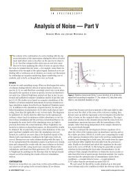
Experimental - Spectroscopy
Experimental - Spectroscopy
Experimental - Spectroscopy

Create successful ePaper yourself
Turn your PDF publications into a flip-book with our unique Google optimized e-Paper software.
18 <strong>Spectroscopy</strong> 26(6) June 2011<br />
www.spectroscopyonline.com<br />
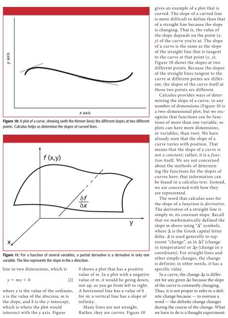
y axis<br />
line in two dimensions, which is<br />
y = mx + b [2]<br />
where y is the value of the ordinate,<br />
x is the value of the abscissa, m is<br />
the slope, and b is the y-intercept,<br />
which is where the plot would<br />
intersect with the y axis. Figure<br />
x axis<br />
Figure 10: A plot of a curve, showing (with the thinner lines) the different slopes at two different<br />
points. Calculus helps us determine the slopes of curved lines.<br />
x<br />
f (x,y)<br />
δf<br />
δx<br />
Figure 11: For a function of several variables, a partial derivative is a derivative in only one<br />
variable. The line represents the slope in the x direction.<br />
9 shows a plot that has a positive<br />
value of m. In a plot with a negative<br />
value of m, it would be going down,<br />
not up, as you go from left to right.<br />
A horizontal line has a value of 0<br />
for m; a vertical line has a slope of<br />
infinity.<br />
Many lines are not straight.<br />
Rather, they are curves. Figure 10<br />
y<br />
gives an example of a plot that is<br />
curved. The slope of a curved line<br />
is more difficult to define than that<br />
of a straight line because the slope<br />
is changing. That is, the value of<br />
the slope depends on the point (x,<br />
y) of the curve you’re at. The slope<br />
of a curve is the same as the slope<br />
of the straight line that is tangent<br />
to the curve at that point (x, y).<br />
Figure 10 shows the slopes at two<br />
different points. Because the slopes<br />
of the straight lines tangent to the<br />
curve at different points are different,<br />
the slopes of the curve itself at<br />
those two points are different.<br />
Calculus provides ways of determining<br />
the slope of a curve, in any<br />
number of dimensions (Figure 10 is<br />
a two-dimensional plot, but we recognize<br />
that functions can be functions<br />
of more than one variable, so<br />
plots can have more dimensions,<br />
or variables, than two). We have<br />
already seen that the slope of a<br />
curve varies with position. That<br />
means that the slope of a curve is<br />
not a constant; rather, it is a function<br />
itself. We are not concerned<br />
about the methods of determining<br />
the functions for the slopes of<br />
curves here; that information can<br />
be found in a calculus text. Instead,<br />
we are concerned with how they<br />
are represented.<br />
The word that calculus uses for<br />
the slope of a function is derivative.<br />
The derivative of a straight line is<br />
simply m, its constant slope. Recall<br />
that we mathematically defined the<br />
slope m above using “Δ” symbols,<br />
where Δ is the Greek capital letter<br />
delta. Δ is used generally to represent<br />
“change”, as in ΔT (change<br />
in temperature) or Δy (change in y<br />
coordinate). For straight lines and<br />
other simple changes, the change<br />
is definite; in other words, it has a<br />
specific value.<br />
In a curve, the change Δy is different<br />
for any given Δx because the slope<br />
of the curve is constantly changing.<br />
Thus, it is not proper to refer to a definite<br />
change because — to overuse a<br />
word — the definite change changes<br />
during the course of the change. What<br />
we have to do is a thought experiment: