

arch postestimation - Stata
arch postestimation - Stata
arch postestimation - Stata

Create successful ePaper yourself
Turn your PDF publications into a flip-book with our unique Google optimized e-Paper software.
2 <strong>arch</strong> <strong>postestimation</strong> — Postestimation tools for <strong>arch</strong><br />
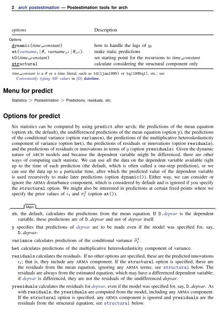
options<br />
Options<br />
dynamic(time constant)<br />
at(varname ɛ | # ɛ varname σ 2 | # σ 2)<br />
t0(time constant)<br />
structural<br />
Description<br />
how to handle the lags of y t<br />
make static predictions<br />
set starting point for the recursions to time constant<br />
calculate considering the structural component only<br />
time constant is a # or a time literal, such as td(1jan1995) or tq(1995q1), etc.; see<br />
Conveniently typing SIF values in [D] datetime.<br />
Menu for predict<br />
Statistics > Postestimation > Predictions, residuals, etc.<br />
Options for predict<br />
Six statistics can be computed by using predict after <strong>arch</strong>: the predictions of the mean equation<br />
(option xb, the default), the undifferenced predictions of the mean equation (option y), the predictions<br />
of the conditional variance (option variance), the predictions of the multiplicative heteroskedasticity<br />
component of variance (option het), the predictions of residuals or innovations (option residuals),<br />
and the predictions of residuals or innovations in terms of y (option yresiduals). Given the dynamic<br />
nature of ARCH models and because the dependent variable might be differenced, there are other<br />
ways of computing each statistic. We can use all the data on the dependent variable available right<br />
up to the time of each prediction (the default, which is often called a one-step prediction), or we<br />
can use the data up to a particular time, after which the predicted value of the dependent variable<br />
is used recursively to make later predictions (option dynamic()). Either way, we can consider or<br />
ignore the ARMA disturbance component, which is considered by default and is ignored if you specify<br />
the structural option. We might also be interested in predictions at certain fixed points where we<br />
specify the prior values of ɛ t and σt<br />
2 (option at()).<br />
✄<br />
✄<br />
Main<br />
<br />
xb, the default, calculates the predictions from the mean equation. If D.depvar is the dependent<br />
variable, these predictions are of D.depvar and not of depvar itself.<br />
y specifies that predictions of depvar are to be made even if the model was specified for, say,<br />
D.depvar.<br />
variance calculates predictions of the conditional variance ̂σ 2 t .<br />
het calculates predictions of the multiplicative heteroskedasticity component of variance.<br />
residuals calculates the residuals. If no other options are specified, these are the predicted innovations<br />
ɛ t ; that is, they include any ARMA component. If the structural option is specified, these are<br />
the residuals from the mean equation, ignoring any ARMA terms; see structural below. The<br />
residuals are always from the estimated equation, which may have a differenced dependent variable;<br />
if depvar is differenced, they are not the residuals of the undifferenced depvar.<br />
yresiduals calculates the residuals for depvar, even if the model was specified for, say, D.depvar. As<br />
with residuals, the yresiduals are computed from the model, including any ARMA component.<br />
If the structural option is specified, any ARMA component is ignored and yresiduals are the<br />
residuals from the structural equation; see structural below.


