logit - Stata

Title 

stata.com 

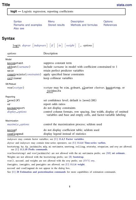
logit — Logistic regression, reporting coefficients 

Syntax Menu Description Options 

Remarks and examples Stored results Methods and formulas References 

Also see 

Syntax 

logit depvar [ indepvars ] [ if ] [ in ] [ weight ] [ , options ] 

options 

Description 

Model 

noconstant 

suppress constant term 

offset(varname) include varname in model with coefficient constrained to 1 

asis 

retain perfect predictor variables 

constraints(constraints) apply specified linear constraints 

collinear 

keep collinear variables 

SE/Robust 

vce(vcetype) 

Reporting 

level(#) 

or 

nocnsreport 

display options 

vcetype may be oim, robust, cluster clustvar, bootstrap, or 

jackknife 

set confidence level; default is level(95) 

report odds ratios 

do not display constraints 

control column formats, row spacing, line width, display of omitted 

variables and base and empty cells, and factor-variable labeling 

Maximization 

maximize options 

nocoef 

coeflegend 

control the maximization process; seldom used 

do not display coefficient table; seldom used 

display legend instead of statistics 

indepvars may contain factor variables; see [U] 11.4.3 Factor variables. 

depvar and indepvars may contain time-series operators; see [U] 11.4.4 Time-series varlists. 

bootstrap, by, fp, jackknife, mfp, mi estimate, nestreg, rolling, statsby, stepwise, and svy are allowed; 

see [U] 11.1.10 Prefix commands. 

vce(bootstrap) and vce(jackknife) are not allowed with the mi estimate prefix; see [MI] mi estimate. 

Weights are not allowed with the bootstrap prefix; see [R] bootstrap. 

vce(), nocoef, and weights are not allowed with the svy prefix; see [SVY] svy. 

fweights, iweights, and pweights are allowed; see [U] 11.1.6 weight. 

nocoef and coeflegend do not appear in the dialog box. 

See [U] 20 Estimation and postestimation commands for more capabilities of estimation commands. 

1

2 logit — Logistic regression, reporting coefficients 

Menu 

Statistics > Binary outcomes > Logistic regression 

Description 

logit fits a logit model for a binary response by maximum likelihood; it models the probability 

of a positive outcome given a set of regressors. depvar equal to nonzero and nonmissing (typically 

depvar equal to one) indicates a positive outcome, whereas depvar equal to zero indicates a negative 

outcome. 

Also see [R] logistic; logistic displays estimates as odds ratios. Many users prefer the logistic 

command to logit. Results are the same regardless of which you use—both are the maximumlikelihood 

estimator. Several auxiliary commands that can be run after logit, probit, or logistic 

estimation are described in [R] logistic postestimation. A list of related estimation commands is given 

in [R] logistic. 

Options 

✄ 

✄ 

✄ 

✄ 

If estimating on grouped data, see [R] glogit. 

✄ 

Model 

 

noconstant, offset(varname), constraints(constraints), collinear; see [R] estimation options. 

asis forces retention of perfect predictor variables and their associated perfectly predicted observations 

and may produce instabilities in maximization; see [R] probit. 

✄ 

SE/Robust 

 

vce(vcetype) specifies the type of standard error reported, which includes types that are derived 

from asymptotic theory (oim), that are robust to some kinds of misspecification (robust), that 

allow for intragroup correlation (cluster clustvar), and that use bootstrap or jackknife methods 

(bootstrap, jackknife); see [R] vce option. 

✄ 

Reporting 

 

level(#); see [R] estimation options. 

or reports the estimated coefficients transformed to odds ratios, that is, e b rather than b. Standard errors 

and confidence intervals are similarly transformed. This option affects how results are displayed, 

not how they are estimated. or may be specified at estimation or when replaying previously 

estimated results. 

nocnsreport; see [R] estimation options. 

display options: noomitted, vsquish, noemptycells, baselevels, allbaselevels, nofvlabel, 

fvwrap(#), fvwrapon(style), cformat(% fmt), pformat(% fmt), sformat(% fmt), and 

nolstretch; see [R] estimation options. 

✄ 

Maximization 

 

maximize options: difficult, technique(algorithm spec), iterate(#), [ no ] log, trace, 

gradient, showstep, hessian, showtolerance, tolerance(#), ltolerance(#), 

nrtolerance(#), nonrtolerance, and from(init specs); see [R] maximize. These options are 

seldom used.

logit — Logistic regression, reporting coefficients 3 

The following options are available with logit but are not shown in the dialog box: 

nocoef specifies that the coefficient table not be displayed. This option is sometimes used by program 

writers but is of no use interactively. 

coeflegend; see [R] estimation options. 

Remarks and examples 

Remarks are presented under the following headings: 

Basic usage 

Model identification 

stata.com 

Basic usage 

logit fits maximum likelihood models with dichotomous dependent (left-hand-side) variables 

coded as 0/1 (or, more precisely, coded as 0 and not-0). 

Example 1 

We have data on the make, weight, and mileage rating of 22 foreign and 52 domestic automobiles. 

We wish to fit a logit model explaining whether a car is foreign on the basis of its weight and mileage. 

Here is an overview of our data: 

. use http://www.stata-press.com/data/r13/auto 

(1978 Automobile Data) 

. keep make mpg weight foreign 

. describe 

Contains data from http://www.stata-press.com/data/r13/auto.dta 

obs: 74 1978 Automobile Data 

vars: 4 13 Apr 2013 17:45 

size: 1,702 (_dta has notes) 

storage display value 

variable name type format label variable label 

make str18 %-18s Make and Model 

mpg int %8.0g Mileage (mpg) 

weight int %8.0gc Weight (lbs.) 

foreign byte %8.0g origin Car type 

Sorted by: foreign 

Note: dataset has changed since last saved 

. inspect foreign 

foreign: Car type Number of Observations 

Total Integers Nonintegers 

# Negative - - - 

# Zero 52 52 - 

# Positive 22 22 - 

# 

# # Total 74 74 - 

# # Missing - 

0 1 74 

(2 unique values) 

foreign is labeled and all values are documented in the label.


The variable foreign takes on two unique values, 0 and 1. The value 0 denotes a domestic car, 

and 1 denotes a foreign car. 

The model that we wish to fit is 

Pr(foreign = 1) = F (β 0 + β 1 weight + β 2 mpg) 

where F (z) = e z /(1 + e z ) is the cumulative logistic distribution. 

To fit this model, we type 

. logit foreign weight mpg 

Iteration 0: log likelihood = -45.03321 






Logistic regression Number of obs = 74 

LR chi2(2) = 35.72 

Prob > chi2 = 0.0000 

Log likelihood = -27.175156 Pseudo R2 = 0.3966 

foreign Coef. Std. Err. z P>|z| [95% Conf. Interval] 

weight -.0039067 .0010116 -3.86 0.000 -.0058894 -.001924 

mpg -.1685869 .0919175 -1.83 0.067 -.3487418 .011568 

_cons 13.70837 4.518709 3.03 0.002 4.851859 22.56487 

We find that heavier cars are less likely to be foreign and that cars yielding better gas mileage are 

also less likely to be foreign, at least holding the weight of the car constant. 

Technical note 

Stata interprets a value of 0 as a negative outcome (failure) and treats all other values (except 

missing) as positive outcomes (successes). Thus if your dependent variable takes on the values 0 and 

1, then 0 is interpreted as failure and 1 as success. If your dependent variable takes on the values 0, 

1, and 2, then 0 is still interpreted as failure, but both 1 and 2 are treated as successes. 

If you prefer a more formal mathematical statement, when you type logit y x, Stata fits the 

model 

Pr(y j ≠ 0 | x j ) = 

exp(x jβ) 

1 + exp(x j β) 

Model identification 

The logit command has one more feature, and it is probably the most useful. logit automatically 

checks the model for identification and, if it is underidentified, drops whatever variables and observations 

are necessary for estimation to proceed. (logistic, probit, and ivprobit do this as well.)


Example 2 

Have you ever fit a logit model where one or more of your independent variables perfectly predicted 

one or the other outcome? 

For instance, consider the following data: 

Outcome y 

Independent variable x 

0 1 

0 1 

0 0 

1 0 

Say that we wish to predict the outcome on the basis of the independent variable. The outcome is 

always zero whenever the independent variable is one. In our data, Pr(y = 0 | x = 1) = 1, which 

means that the logit coefficient on x must be minus infinity with a corresponding infinite standard 

error. At this point, you may suspect that we have a problem. 

Unfortunately, not all such problems are so easily detected, especially if you have a lot of 

independent variables in your model. If you have ever had such difficulties, you have experienced one 

of the more unpleasant aspects of computer optimization. The computer has no idea that it is trying 

to solve for an infinite coefficient as it begins its iterative process. All it knows is that at each step, 

making the coefficient a little bigger, or a little smaller, works wonders. It continues on its merry 

way until either 1) the whole thing comes crashing to the ground when a numerical overflow error 

occurs or 2) it reaches some predetermined cutoff that stops the process. In the meantime, you have 

been waiting. The estimates that you finally receive, if you receive any at all, may be nothing more 

than numerical roundoff. 

Stata watches for these sorts of problems, alerts us, fixes them, and properly fits the model. 

Let’s return to our automobile data. Among the variables we have in the data is one called repair, 

which takes on three values. A value of 1 indicates that the car has a poor repair record, 2 indicates 

an average record, and 3 indicates a better-than-average record. Here is a tabulation of our data: 

. use http://www.stata-press.com/data/r13/repair, clear 


. tabulate foreign repair 

repair 

Car type 1 2 3 Total 

Domestic 10 27 9 46 

Foreign 0 3 9 12 

Total 10 30 18 58 

All the cars with poor repair records (repair = 1) are domestic. If we were to attempt to predict 

foreign on the basis of the repair records, the predicted probability for the repair = 1 category 

would have to be zero. This in turn means that the logit coefficient must be minus infinity, and that 

would set most computer programs buzzing.


Let’s try Stata on this problem. 

. logit foreign b3.repair 

note: 1.repair != 0 predicts failure perfectly 

1.repair dropped and 10 obs not used 







LR chi2(1) = 9.53 

Prob > chi2 = 0.0020 



repair 

1 0 (empty) 

2 -2.197225 .7698003 -2.85 0.004 -3.706005 -.6884436 

_cons -1.98e-16 .4714045 -0.00 1.000 -.9239359 .9239359 

Remember that all the cars with poor repair records (repair = 1) are domestic, so the model 

cannot be fit, or at least it cannot be fit if we restrict ourselves to finite coefficients. Stata noted 

that fact “note: 1.repair !=0 predicts failure perfectly”. This is Stata’s mathematically precise way of 

saying what we said in English. When repair is 1, the car is domestic. 

Stata then went on to say “1.repair dropped and 10 obs not used”. This is Stata eliminating 

the problem. First 1.repair had to be removed from the model because it would have an infinite 

coefficient. Then the 10 observations that led to the problem had to be eliminated, as well, so as 

not to bias the remaining coefficients in the model. The 10 observations that are not used are the 10 

domestic cars that have poor repair records. 

Stata then fit what was left of the model, using the remaining observations. Because no observations 

remained for cars with poor repair records, Stata reports “(empty)” in the row for repair = 1. 

Technical note 

Stata is pretty smart about catching problems like this. It will catch “one-way causation by a 

dummy variable”, as we demonstrated above. 

Stata also watches for “two-way causation”, that is, a variable that perfectly determines the 

outcome, both successes and failures. Here Stata says, “so-and-so predicts outcome perfectly” and 

stops. Statistics dictates that no model can be fit. 

Stata also checks your data for collinear variables; it will say, “so-and-so omitted because of 

collinearity”. No observations need to be eliminated in this case, and model fitting will proceed 

without the offending variable. 

It will also catch a subtle problem that can arise with continuous data. For instance, if we were 

estimating the chances of surviving the first year after an operation, and if we included in our model 

age, and if all the persons over 65 died within the year, Stata would say, “age > 65 predicts failure 

perfectly”. It would then inform us about the fix-up it takes and fit what can be fit of our model.


logit (and logistic, probit, and ivprobit) will also occasionally display messages such as 

Note: 4 failures and 0 successes completely determined. 

There are two causes for a message like this. The first—and most unlikely—case occurs when 

a continuous variable (or a combination of a continuous variable with other continuous or dummy 

variables) is simply a great predictor of the dependent variable. Consider Stata’s auto.dta dataset 

with 6 observations removed. 

. use http://www.stata-press.com/data/r13/auto 


. drop if foreign==0 & gear_ratio > 3.1 

(6 observations deleted) 

. logit foreign mpg weight gear_ratio, nolog 


LR chi2(3) = 72.64 

Prob > chi2 = 0.0000 



mpg -.4944907 .2655508 -1.86 0.063 -1.014961 .0259792 

weight -.0060919 .003101 -1.96 0.049 -.0121698 -.000014 

gear_ratio 15.70509 8.166234 1.92 0.054 -.300436 31.71061 

_cons -21.39527 25.41486 -0.84 0.400 -71.20747 28.41694 


There are no missing standard errors in the output. If you receive the “completely determined” message 

and have one or more missing standard errors in your output, see the second case discussed below. 

Note gear ratio’s large coefficient. logit thought that the 4 observations with the smallest 

predicted probabilities were essentially predicted perfectly. 

. predict p 

(option pr assumed; Pr(foreign)) 

. sort p 

. list p in 1/4 

p 

1. 1.34e-10 

2. 6.26e-09 

3. 7.84e-09 

4. 1.49e-08 

If this happens to you, you do not have to do anything. Computationally, the model is sound. The 

second case discussed below requires careful examination. 

The second case occurs when the independent terms are all dummy variables or continuous ones 

with repeated values (for example, age). Here one or more of the estimated coefficients will have 

missing standard errors. For example, consider this dataset consisting of 5 observations.


. use http://www.stata-press.com/data/r13/logitxmpl, clear 

. list, separator(0) 

y x1 x2 

1. 0 0 0 

2. 0 0 0 

3. 0 1 0 

4. 1 1 0 

5. 0 0 1 

6. 1 0 1 

. logit y x1 x2 







(output omitted ) 






convergence not achieved 

(not concave) 

(not concave) 

(not concave) 

(not concave) 

(not concave) 


LR chi2(1) = 2.09 

Prob > chi2 = 0.1480 


y Coef. Std. Err. z P>|z| [95% Conf. Interval] 

x1 18.3704 2 9.19 0.000 14.45047 22.29033 

x2 18.3704 . . . . . 

_cons -18.3704 1.414214 -12.99 0.000 -21.14221 -15.5986 


convergence not achieved 

r(430); 

Three things are happening here. First, logit iterates almost forever and then declares nonconvergence. 

Second, logit can fit the outcome (y = 0) for the covariate pattern x1 = 0 and x2 = 0 (that 

is, the first two observations) perfectly. This observation is the “2 failures and 0 successes completely 

determined”. Third, if this observation is dropped, then x1, x2, and the constant are collinear. 

This is the cause of the nonconvergence, the message “completely determined”, and the missing 

standard errors. It happens when you have a covariate pattern (or patterns) with only one outcome 

and there is collinearity when the observations corresponding to this covariate pattern are dropped. 

If this happens to you, confirm the causes. First, identify the covariate pattern with only one 

outcome. (For your data, replace x1 and x2 with the independent variables of your model.)


. egen pattern = group(x1 x2) 

. quietly logit y x1 x2, iterate(100) 

. predict p 

(option pr assumed; Pr(y)) 

. summarize p 

Variable Obs Mean Std. Dev. Min Max 

p 6 .3333333 .2581989 1.05e-08 .5 

If successes were completely determined, that means that there are predicted probabilities that are 

almost 1. If failures were completely determined, that means that there are predicted probabilities 

that are almost 0. The latter is the case here, so we locate the corresponding value of pattern: 

. tabulate pattern if p < 1e-7 

group(x1 

x2) Freq. Percent Cum. 

1 2 100.00 100.00 

Total 2 100.00 

Once we omit this covariate pattern from the estimation sample, logit can deal with the collinearity: 

. logit y x1 x2 if pattern != 1, nolog 

note: x2 omitted because of collinearity 


LR chi2(1) = 0.00 

Prob > chi2 = 1.0000 



x1 0 2 0.00 1.000 -3.919928 3.919928 

x2 0 (omitted) 

_cons 0 1.414214 0.00 1.000 -2.771808 2.771808 

We omit the collinear variable. Then we must decide whether to include or omit the observations 

with pattern = 1. We could include them, 

. logit y x1, nolog 


LR chi2(1) = 0.37 

Prob > chi2 = 0.5447 



x1 1.098612 1.825742 0.60 0.547 -2.479776 4.677001 

_cons -1.098612 1.154701 -0.95 0.341 -3.361784 1.164559


or exclude them, 

. logit y x1 if pattern != 1, nolog 


LR chi2(1) = 0.00 

Prob > chi2 = 1.0000 



x1 0 2 0.00 1.000 -3.919928 3.919928 

_cons 0 1.414214 0.00 1.000 -2.771808 2.771808 

If the covariate pattern that predicts outcome perfectly is meaningful, you may want to exclude these 

observations from the model. Here you would report that covariate pattern such and such predicted 

outcome perfectly and that the best model for the rest of the data is . . . . But, more likely, the perfect 

prediction was simply the result of having too many predictors in the model. Then you would omit 

the extraneous variables from further consideration and report the best model for all the data. 

Stored results 

logit stores the following in e(): 

Scalars 

e(N) 

number of observations 

e(N cds) 

number of completely determined successes 

e(N cdf) 

number of completely determined failures 

e(k) 

number of parameters 

e(k eq) 

number of equations in e(b) 

e(k eq model) 

number of equations in overall model test 

e(k dv) 

number of dependent variables 

e(df m) 

model degrees of freedom 

e(r2 p) 

pseudo-R-squared 

e(ll) 

log likelihood 

e(ll 0) 

log likelihood, constant-only model 

e(N clust) 

number of clusters 

e(chi2) χ 2 

e(p) 

significance of model test 

e(rank) 

rank of e(V) 

e(ic) 

number of iterations 

e(rc) 

return code 

e(converged) 

1 if converged, 0 otherwise


Macros 

e(cmd) 

logit 

e(cmdline) 

command as typed 

e(depvar) 

name of dependent variable 

e(wtype) 

weight type 

e(wexp) 

weight expression 

e(title) 

title in estimation output 

e(clustvar) 

name of cluster variable 

e(offset) 

linear offset variable 

e(chi2type) Wald or LR; type of model χ 2 test 

e(vce) 

vcetype specified in vce() 

e(vcetype) 

title used to label Std. Err. 

e(opt) 

type of optimization 

e(which) 

max or min; whether optimizer is to perform maximization or minimization 

e(ml method) 

type of ml method 

e(user) 

name of likelihood-evaluator program 

e(technique) 

maximization technique 

e(properties) 

b V 

e(estat cmd) 

program used to implement estat 

e(predict) 

program used to implement predict 

e(marginsnotok) predictions disallowed by margins 

e(asbalanced) 

factor variables fvset as asbalanced 

e(asobserved) 

factor variables fvset as asobserved 

Matrices 

e(b) 

e(Cns) 

e(ilog) 

e(gradient) 

e(mns) 

e(rules) 

e(V) 

e(V modelbased) 

Functions 

e(sample) 

coefficient vector 

constraints matrix 

iteration log (up to 20 iterations) 

gradient vector 

vector of means of the independent variables 

information about perfect predictors 

variance–covariance matrix of the estimators 

model-based variance 

marks estimation sample 

Methods and formulas 

Cramer (2003, chap. 9) surveys the prehistory and history of the logit model. The word “logit” 

was coined by Berkson (1944) and is analogous to the word “probit”. For an introduction to probit 

and logit, see, for example, Aldrich and Nelson (1984), Cameron and Trivedi (2010), Greene (2012), 

Jones (2007), Long (1997), Long and Freese (2006), Pampel (2000), or Powers and Xie (2008). 

The likelihood function for logit is 

lnL = ∑ j∈S 

w j lnF (x j b) + ∑ j∉S 

w j ln { 1 − F (x j b) }


where S is the set of all observations j, such that y j ≠ 0, F (z) = e z /(1 + e z ), and w j denotes the 

optional weights. lnL is maximized as described in [R] maximize. 

This command supports the Huber/White/sandwich estimator of the variance and its clustered version 

using vce(robust) and vce(cluster clustvar), respectively. See [P] robust, particularly Maximum 

likelihood estimators and Methods and formulas. The scores are calculated as u j = {1 − F (x j b)}x j 

for the positive outcomes and −F (x j b)x j for the negative outcomes. 

logit also supports estimation with survey data. For details on VCEs with survey data, see 

[SVY] variance estimation. 

✄ 

✂ 

Joseph Berkson (1899–1982) was born in New York City and studied at the College of the City 

of New York, Columbia, and Johns Hopkins, earning both an MD and a doctorate in statistics. 

He then worked at Johns Hopkins before moving to the Mayo Clinic in 1931 as a biostatistician. 

Among many other contributions, his most influential one drew upon a long-sustained interest 

in the logistic function, especially his 1944 paper on bioassay, in which he introduced the term 

“logit”. Berkson was a frequent participant in controversy—sometimes humorous, sometimes 

bitter—on subjects such as the evidence for links between smoking and various diseases and the 

relative merits of probit and logit methods and of different calculation methods. 

 

✁ 

References 

Aldrich, J. H., and F. D. Nelson. 1984. Linear Probability, Logit, and Probit Models. Newbury Park, CA: Sage. 

Archer, K. J., and S. A. Lemeshow. 2006. Goodness-of-fit test for a logistic regression model fitted using survey 

sample data. Stata Journal 6: 97–105. 

Berkson, J. 1944. Application of the logistic function to bio-assay. Journal of the American Statistical Association 

39: 357–365. 

Buis, M. L. 2010a. Direct and indirect effects in a logit model. Stata Journal 10: 11–29. 

. 2010b. Stata tip 87: Interpretation of interactions in nonlinear models. Stata Journal 10: 305–308. 

Cameron, A. C., and P. K. Trivedi. 2010. Microeconometrics Using Stata. Rev. ed. College Station, TX: Stata Press. 

Cleves, M. A., and A. Tosetto. 2000. sg139: Logistic regression when binary outcome is measured with uncertainty. 

Stata Technical Bulletin 55: 20–23. Reprinted in Stata Technical Bulletin Reprints, vol. 10, pp. 152–156. College 

Station, TX: Stata Press. 

Cramer, J. S. 2003. Logit Models from Economics and Other Fields. Cambridge: Cambridge University Press. 

Greene, W. H. 2012. Econometric Analysis. 7th ed. Upper Saddle River, NJ: Prentice Hall. 

Hilbe, J. M. 2009. Logistic Regression Models. Boca Raton, FL: Chapman & Hill/CRC. 

Hosmer, D. W., Jr., S. A. Lemeshow, and R. X. Sturdivant. 2013. Applied Logistic Regression. 3rd ed. Hoboken, 

NJ: Wiley. 

Jones, A. 2007. Applied Econometrics for Health Economists: A Practical Guide. 2nd ed. Abingdon, UK: Radcliffe. 

Judge, G. G., W. E. Griffiths, R. C. Hill, H. Lütkepohl, and T.-C. Lee. 1985. The Theory and Practice of Econometrics. 

2nd ed. New York: Wiley. 

Long, J. S. 1997. Regression Models for Categorical and Limited Dependent Variables. Thousand Oaks, CA: Sage. 

Long, J. S., and J. Freese. 2006. Regression Models for Categorical Dependent Variables Using Stata. 2nd ed. College 

Station, TX: Stata Press. 

Miranda, A., and S. Rabe-Hesketh. 2006. Maximum likelihood estimation of endogenous switching and sample 

selection models for binary, ordinal, and count variables. Stata Journal 6: 285–308. 

Mitchell, M. N., and X. Chen. 2005. Visualizing main effects and interactions for binary logit models. Stata Journal 

5: 64–82.


O’Fallon, W. M. 1998. Berkson, Joseph. In Vol. 1 of Encyclopedia of Biostatistics, ed. P. Armitage and T. Colton, 

290–295. Chichester, UK: Wiley. 

Orsini, N., R. Bellocco, and P. C. Sjölander. 2013. Doubly robust estimation in generalized linear models. Stata 

Journal 13: 185–205. 

Pampel, F. C. 2000. Logistic Regression: A Primer. Thousand Oaks, CA: Sage. 

Powers, D. A., and Y. Xie. 2008. Statistical Methods for Categorical Data Analysis. 2nd ed. Bingley, UK: Emerald. 

Pregibon, D. 1981. Logistic regression diagnostics. Annals of Statistics 9: 705–724. 

Schonlau, M. 2005. Boosted regression (boosting): An introductory tutorial and a Stata plugin. Stata Journal 5: 

330–354. 

Xu, J., and J. S. Long. 2005. Confidence intervals for predicted outcomes in regression models for categorical 

outcomes. Stata Journal 5: 537–559. 

Also see 

[R] logit postestimation — Postestimation tools for logit 

[R] brier — Brier score decomposition 

[R] cloglog — Complementary log-log regression 

[R] exlogistic — Exact logistic regression 

[R] glogit — Logit and probit regression for grouped data 

[R] logistic — Logistic regression, reporting odds ratios 

[R] probit — Probit regression 

[R] roc — Receiver operating characteristic (ROC) analysis 

[ME] melogit — Multilevel mixed-effects logistic regression 

[MI] estimation — Estimation commands for use with mi estimate 

[SVY] svy estimation — Estimation commands for survey data 

[XT] xtlogit — Fixed-effects, random-effects, and population-averaged logit models 

[U] 20 Estimation and postestimation commands

logit - Stata

Create successful ePaper yourself

Delete template?

Save as template?