xtlogit - Stata

Title
stata.com
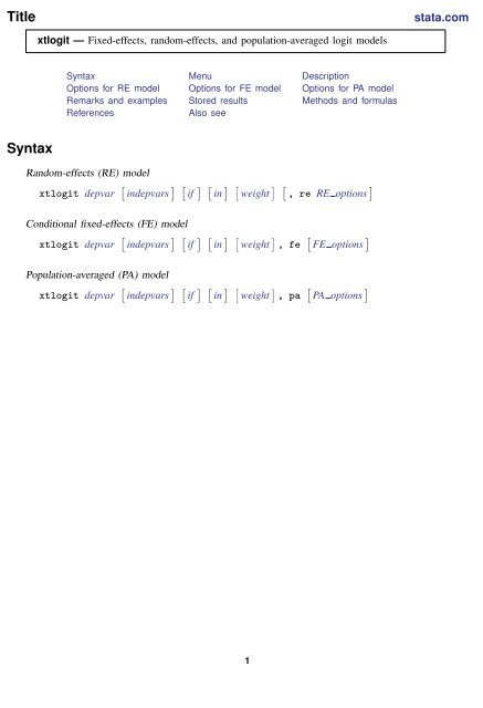
xtlogit — Fixed-effects, random-effects, and population-averaged logit models
Syntax Menu Description
Options for RE model Options for FE model Options for PA model
Remarks and examples Stored results Methods and formulas
References
Also see
Syntax
Random-effects (RE) model
xtlogit depvar [ indepvars ] [ if ] [ in ] [ weight ] [ , re RE options ]
Conditional fixed-effects (FE) model
xtlogit depvar [ indepvars ] [ if ] [ in ] [ weight ] , fe [ FE options ]
Population-averaged (PA) model
xtlogit depvar [ indepvars ] [ if ] [ in ] [ weight ] , pa [ PA options ]
1

2 xtlogit — Fixed-effects, random-effects, and population-averaged logit models
RE options
Description
Model
noconstant
suppress constant term
re
use random-effects estimator; the default
offset(varname) include varname in model with coefficient constrained to 1
constraints(constraints) apply specified linear constraints
collinear
keep collinear variables
asis
retain perfect predictor variables
SE/Robust
vce(vcetype)
Reporting
level(#)
or
noskip
nocnsreport
display options
Integration
intmethod(intmethod)
intpoints(#)
Maximization
maximize options
nodisplay
coeflegend
vcetype may be oim, robust, cluster clustvar, bootstrap, or
jackknife
set confidence level; default is level(95)
report odds ratios
perform overall model test as a likelihood-ratio test
do not display constraints
control column formats, row spacing, line width, display of omitted
variables and base and empty cells, and factor-variable labeling
integration method; intmethod may be mvaghermite (the default) or
ghermite
use # quadrature points; default is intpoints(12)
control the maximization process; seldom used
suppress display of header and coefficients
display legend instead of statistics

xtlogit — Fixed-effects, random-effects, and population-averaged logit models 3
FE options
Description
Model
fe
use fixed-effects estimator
offset(varname) include varname in model with coefficient constrained to 1
constraints(constraints) apply specified linear constraints
collinear
keep collinear variables
SE
vce(vcetype)
Reporting
level(#)
or
noskip
nocnsreport
display options
Maximization
maximize options
nodisplay
coeflegend
vcetype may be oim, bootstrap, or jackknife
set confidence level; default is level(95)
report odds ratios
perform overall model test as a likelihood-ratio test
do not display constraints
control column formats, row spacing, line width, display of omitted
variables and base and empty cells, and factor-variable labeling
control the maximization process; seldom used
suppress display of header and coefficients
display legend instead of statistics

4 xtlogit — Fixed-effects, random-effects, and population-averaged logit models
PA options
Description
Model
noconstant
suppress constant term
pa
use population-averaged estimator
offset(varname) include varname in model with coefficient constrained to 1
asis
retain perfect predictor variables
Correlation
corr(correlation)
force
SE/Robust
vce(vcetype)
nmp
scale(parm)
Reporting
level(#)
or
display options
Optimization
optimize options
nodisplay
coeflegend
within-panel correlation structure
estimate even if observations unequally spaced in time
vcetype may be conventional, robust, bootstrap, or
jackknife
use divisor N − P instead of the default N
overrides the default scale parameter;
parm may be x2, dev, phi, or #
set confidence level; default is level(95)
report odds ratios
control column formats, row spacing, line width, display of omitted
variables and base and empty cells, and factor-variable labeling
control the optimization process; seldom used
do not display the header and coefficients
display legend instead of statistics
correlation
Description
exchangeable
exchangeable
independent
independent
unstructured
unstructured
fixed matname
user-specified
ar # autoregressive of order #
stationary # stationary of order #
nonstationary # nonstationary of order #

xtlogit — Fixed-effects, random-effects, and population-averaged logit models 5
A panel variable must be specified. For xtlogit, pa, correlation structures other than exchangeable and independent
require that a time variable also be specified. Use xtset; see [XT] xtset.
indepvars may contain factor variables; see [U] 11.4.3 Factor variables.
depvar and indepvars may contain time-series operators; see [U] 11.4.4 Time-series varlists.
by, mi estimate, and statsby are allowed; see [U] 11.1.10 Prefix commands. fp is allowed for the random-effects
and fixed-effects models.
vce(bootstrap) and vce(jackknife) are not allowed with the mi estimate prefix; see [MI] mi estimate.
iweights, fweights, and pweights are allowed for the population-averaged model, and iweights are allowed for
the fixed-effects and random-effects models; see [U] 11.1.6 weight. Weights must be constant within panel.
nodisplay and coeflegend do not appear in the dialog box.
See [U] 20 Estimation and postestimation commands for more capabilities of estimation commands.
Menu
Statistics > Longitudinal/panel data > Binary outcomes > Logistic regression (FE, RE, PA)
Description
xtlogit fits random-effects, conditional fixed-effects, and population-averaged logit models.
Whenever we refer to a fixed-effects model, we mean the conditional fixed-effects model. depvar
equal to nonzero and nonmissing (typically depvar equal to one) indicates a positive outcome, whereas
depvar equal to zero indicates a negative outcome.
By default, the population-averaged model is an equal-correlation model; xtlogit, pa assumes
corr(exchangeable). See [XT] xtgee for information on how to fit other population-averaged
models.
See [R] logistic for a list of related estimation commands.
Options for RE model
✄
✄ Model
noconstant; see [R] estimation options.
✄
re requests the random-effects estimator, which is the default.
offset(varname) constraints(constraints), collinear; see [R] estimation options.
asis forces retention of perfect predictor variables and their associated, perfectly predicted observations
and may produce instabilities in maximization; see [R] probit.
✄
SE/Robust
vce(vcetype) specifies the type of standard error reported, which includes types that are derived
from asymptotic theory (oim), that are robust to some kinds of misspecification (robust), that
allow for intragroup correlation (cluster clustvar), and that use bootstrap or jackknife methods
(bootstrap, jackknife); see [XT] vce options.
Specifying vce(robust) is equivalent to specifying vce(cluster panelvar); see xtlogit, re and
the robust VCE estimator in Methods and formulas.
✄
✄ Reporting
level(#); see [R] estimation options.

6 xtlogit — Fixed-effects, random-effects, and population-averaged logit models
or reports the estimated coefficients transformed to odds ratios, that is, e b rather than b. Standard errors
and confidence intervals are similarly transformed. This option affects how results are displayed,
not how they are estimated. or may be specified at estimation or when replaying previously
estimated results.
noskip; see [R] estimation options.
nocnsreport; see [R] estimation options.
display options: noomitted, vsquish, noemptycells, baselevels, allbaselevels, nofvlabel,
fvwrap(#), fvwrapon(style), cformat(% fmt), pformat(% fmt), sformat(% fmt), and
nolstretch; see [R] estimation options.
✄
✄ Integration
intmethod(intmethod), intpoints(#); see [R] estimation options.
✄
✄
Maximization
maximize options: difficult, technique(algorithm spec), iterate(#), [ no ] log, trace,
gradient, showstep, hessian, showtolerance, tolerance(#), ltolerance(#),
nrtolerance(#), nonrtolerance, and from(init specs); see [R] maximize. These options are
seldom used.
The following options are available with xtlogit but are not shown in the dialog box:
nodisplay is for programmers. It suppresses the display of the header and the coefficients.
coeflegend; see [R] estimation options.
Options for FE model
✄
✄ Model
fe requests the fixed-effects estimator.
offset(varname), constraints(constraints), collinear; see [R] estimation options.
✄
✄
SE
vce(vcetype) specifies the type of standard error reported, which includes types that are derived from
asymptotic theory (oim) and that use bootstrap or jackknife methods (bootstrap, jackknife);
see [XT] vce options.
✄
✄ Reporting
level(#); see [R] estimation options.
or reports the estimated coefficients transformed to odds ratios, that is, e b rather than b. Standard errors
and confidence intervals are similarly transformed. This option affects how results are displayed,
not how they are estimated. or may be specified at estimation or when replaying previously
estimated results.
noskip; see [R] estimation options.
nocnsreport; see [R] estimation options.

xtlogit — Fixed-effects, random-effects, and population-averaged logit models 7
✄
display options: noomitted, vsquish, noemptycells, baselevels, allbaselevels, nofvlabel,
fvwrap(#), fvwrapon(style), cformat(% fmt), pformat(% fmt), sformat(% fmt), and
nolstretch; see [R] estimation options.
✄
Maximization
maximize options: difficult, technique(algorithm spec), iterate(#), [ no ] log, trace,
gradient, showstep, hessian, showtolerance, tolerance(#), ltolerance(#),
nrtolerance(#), nonrtolerance, and from(init specs); see [R] maximize. These options are
seldom used.
The following options are available with xtlogit but are not shown in the dialog box:
nodisplay is for programmers. It suppresses the display of the header and the coefficients.
coeflegend; see [R] estimation options.
Options for PA model
✄
✄ Model
noconstant; see [R] estimation options.
✄
✄
pa requests the population-averaged estimator.
offset(varname); see [R] estimation options.
asis forces retention of perfect predictor variables and their associated, perfectly predicted observations
and may produce instabilities in maximization; see [R] probit.
✄
Correlation
corr(correlation) specifies the within-panel correlation structure; the default corresponds to the
equal-correlation model, corr(exchangeable).
When you specify a correlation structure that requires a lag, you indicate the lag after the structure’s
name with or without a blank; for example, corr(ar 1) or corr(ar1).
If you specify the fixed correlation structure, you specify the name of the matrix containing the
assumed correlations following the word fixed, for example, corr(fixed myr).
force specifies that estimation be forced even though the time variable is not equally spaced.
This is relevant only for correlation structures that require knowledge of the time variable. These
correlation structures require that observations be equally spaced so that calculations based on lags
correspond to a constant time change. If you specify a time variable indicating that observations
are not equally spaced, the (time dependent) model will not be fit. If you also specify force,
the model will be fit, and it will be assumed that the lags based on the data ordered by the time
variable are appropriate.
✄
SE/Robust
vce(vcetype) specifies the type of standard error reported, which includes types that are derived from
asymptotic theory (conventional), that are robust to some kinds of misspecification (robust),
and that use bootstrap or jackknife methods (bootstrap, jackknife); see [XT] vce options.
vce(conventional), the default, uses the conventionally derived variance estimator for generalized
least-squares regression.
nmp, scale(x2 | dev | phi | #); see [XT] vce options.

8 xtlogit — Fixed-effects, random-effects, and population-averaged logit models
✄
✄ Reporting
level(#); see [R] estimation options.
or reports the estimated coefficients transformed to odds ratios, that is, e b rather than b. Standard errors
and confidence intervals are similarly transformed. This option affects how results are displayed,
not how they are estimated. or may be specified at estimation or when replaying previously
estimated results.
display options: noomitted, vsquish, noemptycells, baselevels, allbaselevels, nofvlabel,
fvwrap(#), fvwrapon(style), cformat(% fmt), pformat(% fmt), sformat(% fmt), and
nolstretch; see [R] estimation options.
✄
✄ Optimization
optimize options control the iterative optimization process. These options are seldom used.
iterate(#) specifies the maximum number of iterations. When the number of iterations equals #,
the optimization stops and presents the current results, even if convergence has not been reached.
The default is iterate(100).
tolerance(#) specifies the tolerance for the coefficient vector. When the relative change in the
coefficient vector from one iteration to the next is less than or equal to #, the optimization process
is stopped. tolerance(1e-6) is the default.
nolog suppresses display of the iteration log.
trace specifies that the current estimates be printed at each iteration.
The following options are available with xtlogit but are not shown in the dialog box:
nodisplay is for programmers. It suppresses the display of the header and the coefficients.
coeflegend; see [R] estimation options.
Remarks and examples
stata.com
xtlogit is a convenience command if you want the population-averaged model. Typing
. xtlogit . . ., pa . . .
is equivalent to typing
. xtgee . . ., . . . family(binomial) link(logit) corr(exchangeable)
It is also a convenience command if you want the fixed-effects model. Typing
. xtlogit . . ., fe . . .
is equivalent to typing
. clogit . . ., group(varname i) . . .
See also [XT] xtgee and [R] clogit for information about xtlogit.
By default or when re is specified, xtlogit fits via maximum likelihood the random-effects
model
Pr(y it ≠ 0|x it ) = P (x it β + ν i )
for i = 1, . . . , n panels, where t = 1, . . . , n i , ν i are i.i.d., N(0, σ 2 ν), and P (z) = {1 + exp(−z)} −1 .

xtlogit — Fixed-effects, random-effects, and population-averaged logit models 9
Underlying this model is the variance components model
y it ≠ 0 ⇐⇒ x it β + ν i + ɛ it > 0
where ɛ it are i.i.d. logistic distributed with mean zero and variance σ 2 ɛ = π 2 /3, independently of ν i .
Example 1
We are studying unionization of women in the United States and are using the union dataset; see
[XT] xt. We wish to fit a random-effects model of union membership:
. use http://www.stata-press.com/data/r13/union
(NLS Women 14-24 in 1968)
. xtlogit union age grade not_smsa south##c.year
(output omitted )
Random-effects logistic regression Number of obs = 26200
Group variable: idcode Number of groups = 4434
Random effects u_i ~ Gaussian Obs per group: min = 1
avg = 5.9
max = 12
Integration method: mvaghermite Integration points = 12
Wald chi2(6) = 227.46
Log likelihood = -10540.274 Prob > chi2 = 0.0000
union Coef. Std. Err. z P>|z| [95% Conf. Interval]
age .0156732 .0149895 1.05 0.296 -.0137056 .045052
grade .0870851 .0176476 4.93 0.000 .0524965 .1216738
not_smsa -.2511884 .0823508 -3.05 0.002 -.4125929 -.0897839
1.south -2.839112 .6413116 -4.43 0.000 -4.096059 -1.582164
year -.0068604 .0156575 -0.44 0.661 -.0375486 .0238277
south#c.year
1 .0238506 .0079732 2.99 0.003 .0082235 .0394777
_cons -3.009365 .8414963 -3.58 0.000 -4.658667 -1.360062
/lnsig2u 1.749366 .0470017 1.657245 1.841488
sigma_u 2.398116 .0563577 2.290162 2.511158
rho .6361098 .0108797 .6145307 .6571548
Likelihood-ratio test of rho=0: chibar2(01) = 6004.43 Prob >= chibar2 = 0.000
The output includes the additional panel-level variance component. This is parameterized as the log
of the variance ln(σ 2 ν) (labeled lnsig2u in the output). The standard deviation σ ν is also included
in the output and labeled sigma u together with ρ (labeled rho),
σ2 ν
ρ =
σν 2 + σɛ
2
which is the proportion of the total variance contributed by the panel-level variance component.
When rho is zero, the panel-level variance component is unimportant, and the panel estimator is
no different from the pooled estimator. A likelihood-ratio test of this is included at the bottom of the
output. This test formally compares the pooled estimator (logit) with the panel estimator.
As an alternative to the random-effects specification, we might want to fit an equal-correlation
logit model:

10 xtlogit — Fixed-effects, random-effects, and population-averaged logit models
. xtlogit union age grade not_smsa south##c.year, pa
Iteration 1: tolerance = .1487877
Iteration 2: tolerance = .00949342
Iteration 3: tolerance = .00040606
Iteration 4: tolerance = .00001602
Iteration 5: tolerance = 6.628e-07
GEE population-averaged model Number of obs = 26200
Group variable: idcode Number of groups = 4434
Link: logit Obs per group: min = 1
Family: binomial avg = 5.9
Correlation: exchangeable max = 12
Wald chi2(6) = 235.08
Scale parameter: 1 Prob > chi2 = 0.0000
union Coef. Std. Err. z P>|z| [95% Conf. Interval]
age .0165893 .0092229 1.80 0.072 -.0014873 .0346659
grade .0600669 .0108343 5.54 0.000 .0388321 .0813016
not_smsa -.1215445 .0483713 -2.51 0.012 -.2163505 -.0267384
1.south -1.857094 .372967 -4.98 0.000 -2.588096 -1.126092
year -.0121168 .0095707 -1.27 0.205 -.030875 .0066413
south#c.year
1 .0160193 .0046076 3.48 0.001 .0069886 .0250501
_cons -1.39755 .5089508 -2.75 0.006 -2.395075 -.4000247
Example 2
xtlogit with the pa option allows a vce(robust) option, so we can obtain the population-averaged
logit estimator with the robust variance calculation by typing
. xtlogit union age grade not_smsa south##c.year, pa vce(robust) nolog
GEE population-averaged model Number of obs = 26200
Group variable: idcode Number of groups = 4434
Link: logit Obs per group: min = 1
Family: binomial avg = 5.9
Correlation: exchangeable max = 12
Wald chi2(6) = 154.88
Scale parameter: 1 Prob > chi2 = 0.0000
(Std. Err. adjusted for clustering on idcode)
Robust
union Coef. Std. Err. z P>|z| [95% Conf. Interval]
age .0165893 .008951 1.85 0.064 -.0009543 .0341329
grade .0600669 .0133193 4.51 0.000 .0339616 .0861722
not_smsa -.1215445 .0613803 -1.98 0.048 -.2418477 -.0012412
1.south -1.857094 .5389238 -3.45 0.001 -2.913366 -.8008231
year -.0121168 .0096998 -1.25 0.212 -.0311282 .0068945
south#c.year
1 .0160193 .0067217 2.38 0.017 .002845 .0291937
_cons -1.39755 .5603767 -2.49 0.013 -2.495868 -.2992317
These standard errors are somewhat larger than those obtained without the vce(robust) option.

xtlogit — Fixed-effects, random-effects, and population-averaged logit models 11
Finally, we can also fit a fixed-effects model to these data (see also [R] clogit for details):
. xtlogit union age grade not_smsa south##c.year, fe
note: multiple positive outcomes within groups encountered.
note: 2744 groups (14165 obs) dropped because of all positive or
all negative outcomes.
Iteration 0: log likelihood = -4516.5881
Iteration 1: log likelihood = -4510.8906
Iteration 2: log likelihood = -4510.888
Iteration 3: log likelihood = -4510.888
Conditional fixed-effects logistic regression Number of obs = 12035
Group variable: idcode Number of groups = 1690
Obs per group: min = 2
avg = 7.1
max = 12
LR chi2(6) = 78.60
Log likelihood = -4510.888 Prob > chi2 = 0.0000
union Coef. Std. Err. z P>|z| [95% Conf. Interval]
age .0710973 .0960536 0.74 0.459 -.1171643 .2593589
grade .0816111 .0419074 1.95 0.051 -.0005259 .163748
not_smsa .0224809 .1131786 0.20 0.843 -.199345 .2443069
1.south -2.856488 .6765694 -4.22 0.000 -4.182539 -1.530436
year -.0636853 .0967747 -0.66 0.510 -.2533602 .1259896
south#c.year
1 .0264136 .0083216 3.17 0.002 .0101036 .0427235
Technical note
The random-effects model is calculated using quadrature, which is an approximation whose accuracy
depends partially on the number of integration points used. We can use the quadchk command to see
if changing the number of integration points affects the results. If the results change, the quadrature
approximation is not accurate given the number of integration points. Try increasing the number
of integration points using the intpoints() option and run quadchk again. Do not attempt to
interpret the results of estimates when the coefficients reported by quadchk differ substantially. See
[XT] quadchk for details and [XT] xtprobit for an example.
Because the xtlogit likelihood function is calculated by Gauss–Hermite quadrature, on large
problems the computations can be slow. Computation time is roughly proportional to the number of
points used for the quadrature.

12 xtlogit — Fixed-effects, random-effects, and population-averaged logit models
Stored results
xtlogit, re stores the following in e():
Scalars
e(N)
number of observations
e(N g)
number of groups
e(N cd)
number of completely determined observations
e(k)
number of parameters
e(k aux)
number of auxiliary parameters
e(k eq)
number of equations in e(b)
e(k eq model)
number of equations in overall model test
e(k dv)
number of dependent variables
e(df m)
model degrees of freedom
e(ll)
log likelihood
e(ll 0)
log likelihood, constant-only model
e(ll c)
log likelihood, comparison model
e(chi2) χ 2
e(chi2 c) χ 2 for comparison test
e(N clust)
number of clusters
e(rho)
ρ
e(sigma u)
panel-level standard deviation
e(n quad)
number of quadrature points
e(g min)
smallest group size
e(g avg)
average group size
e(g max)
largest group size
e(p)
significance
e(rank)
rank of e(V)
e(rank0)
rank of e(V) for constant-only model
e(ic)
number of iterations
e(rc)
return code
e(converged)
1 if converged, 0 otherwise
Macros
e(cmd)
xtlogit
e(cmdline)
command as typed
e(depvar)
name of dependent variable
e(ivar)
variable denoting groups
e(model)
re
e(wtype)
weight type
e(wexp)
weight expression
e(title)
title in estimation output
e(clustvar)
name of cluster variable
e(offset)
linear offset variable
e(chi2type) Wald or LR; type of model χ 2 test
e(chi2 ct) Wald or LR; type of model χ 2 test corresponding to e(chi2 c)
e(vce)
vcetype specified in vce()
e(vcetype)
title used to label Std. Err.
e(intmethod)
integration method
e(distrib)
Gaussian; the distribution of the random effect
e(opt)
type of optimization
e(which)
max or min; whether optimizer is to perform maximization or minimization
e(ml method)
type of ml method
e(user)
name of likelihood-evaluator program
e(technique)
maximization technique
e(properties)
b V
e(predict)
program used to implement predict
e(asbalanced)
factor variables fvset as asbalanced
e(asobserved)
factor variables fvset as asobserved

xtlogit — Fixed-effects, random-effects, and population-averaged logit models 13
Matrices
e(b)
e(Cns)
e(ilog)
e(gradient)
e(V)
e(V modelbased)
Functions
e(sample)
coefficient vector
constraints matrix
iteration log
gradient vector
variance–covariance matrix of the estimators
model-based variance
marks estimation sample
xtlogit, fe stores the following in e():
Scalars
e(N)
number of observations
e(N g)
number of groups
e(N drop)
number of observations dropped because of all positive or all negative outcomes
e(N group drop) number of groups dropped because of all positive or all negative outcomes
e(k)
number of parameters
e(k eq)
number of equations in e(b)
e(k eq model)
number of equations in overall model test
e(k dv)
number of dependent variables
e(df m)
model degrees of freedom
e(r2 p)
pseudo R-squared
e(ll)
log likelihood
e(ll 0)
log likelihood, constant-only model
e(chi2) χ 2
e(g min)
smallest group size
e(g avg)
average group size
e(g max)
largest group size
e(p)
significance
e(rank)
rank of e(V)
e(ic)
number of iterations
e(rc)
return code
e(converged)
1 if converged, 0 otherwise
Macros
e(cmd)
clogit
e(cmd2)
xtlogit
e(cmdline)
command as typed
e(depvar)
name of dependent variable
e(ivar)
variable denoting groups
e(model)
fe
e(wtype)
weight type
e(wexp)
weight expression
e(title)
title in estimation output
e(offset)
linear offset variable
e(chi2type) LR; type of model χ 2 test
e(vce)
vcetype specified in vce()
e(vcetype)
title used to label Std. Err.
e(group)
name of group() variable
e(multiple)
multiple if multiple positive outcomes within groups
e(opt)
type of optimization
e(which)
max or min; whether optimizer is to perform maximization or minimization
e(ml method)
type of ml method
e(user)
name of likelihood-evaluator program
e(technique)
maximization technique
e(properties)
b V
e(predict)
program used to implement predict
e(marginsok)
predictions allowed by margins
e(marginsnotok) predictions disallowed by margins
e(asbalanced)
factor variables fvset as asbalanced
e(asobserved)
factor variables fvset as asobserved

14 xtlogit — Fixed-effects, random-effects, and population-averaged logit models
Matrices
e(b)
e(Cns)
e(ilog)
e(gradient)
e(V)
Functions
e(sample)
coefficient vector
constraints matrix
iteration log
gradient vector
variance–covariance matrix of the estimators
marks estimation sample
xtlogit, pa stores the following in e():
Scalars
e(N)
number of observations
e(N g)
number of groups
e(df m)
model degrees of freedom
e(chi2) χ 2
e(p)
significance
e(df pear) degrees of freedom for Pearson χ 2
e(chi2 dev) χ 2 test of deviance
e(chi2 dis) χ 2 test of deviance dispersion
e(deviance)
deviance
e(dispers)
deviance dispersion
e(phi)
scale parameter
e(g min)
smallest group size
e(g avg)
average group size
e(g max)
largest group size
e(rank)
rank of e(V)
e(tol)
target tolerance
e(dif)
achieved tolerance
e(rc)
return code
Macros
e(cmd)
xtgee
e(cmd2)
xtlogit
e(cmdline)
command as typed
e(depvar)
name of dependent variable
e(ivar)
variable denoting groups
e(tvar)
variable denoting time within groups
e(model)
pa
e(family)
binomial
e(link)
logit; link function
e(corr)
correlation structure
e(scale)
x2, dev, phi, or #; scale parameter
e(wtype)
weight type
e(wexp)
weight expression
e(offset)
linear offset variable
e(chi2type) Wald; type of model χ 2 test
e(vce)
vcetype specified in vce()
e(vcetype)
title used to label Std. Err.
e(nmp)
nmp, if specified
e(properties)
b V
e(predict)
program used to implement predict
e(marginsnotok) predictions disallowed by margins
e(asbalanced)
factor variables fvset as asbalanced
e(asobserved)
factor variables fvset as asobserved
Matrices
e(b)
e(R)
e(V)
Functions
e(sample)
coefficient vector
estimated working correlation matrix
variance–covariance matrix of the estimators
marks estimation sample

Methods and formulas
xtlogit — Fixed-effects, random-effects, and population-averaged logit models 15
xtlogit reports the population-averaged results obtained using xtgee, family(binomial)
link(logit) to obtain estimates. The fixed-effects results are obtained using clogit. See [XT] xtgee
and [R] clogit for details on the methods and formulas.
If we assume a normal distribution, N(0, σ 2 ν), for the random effects ν i ,
Pr(y i1 , . . . , y ini |x i1 , . . . , x ini ) =
∫ ∞
−∞
e −ν2 i /2σ2 ν
√
2πσν
}
∏
F (y it , x it β + ν i ) dν i
{
ni
t=1
where
⎧
1
⎪⎨
1 + exp(−z)
F (y, z) =
1 ⎪⎩
1 + exp(z)
if y ≠ 0
otherwise
The panel-level likelihood l i is given by
l i =
∫ ∞
−∞
e −ν2 i /2σ2 ν
√
2πσν
{
ni
}
∏
F (y it , x it β + ν i ) dν i
t=1
≡
∫ ∞
−∞
g(y it , x it , ν i )dν i
This integral can be approximated with M-point Gauss–Hermite quadrature
This is equivalent to
∫ ∞
−∞
∫ ∞
−∞
e −x2 h(x)dx ≈
f(x)dx ≈
M∑
wmh(a ∗ ∗ m)
m=1
M∑
wm ∗ exp { (a ∗ m) 2} f(a ∗ m)
m=1
where the wm ∗ denote the quadrature weights and the a∗ m denote the quadrature abscissas. The log
likelihood, L, is the sum of the logs of the panel-level likelihoods l i .
The default approximation of the log likelihood is by adaptive Gauss–Hermite quadrature, which
approximates the panel-level likelihood with
l i ≈ √ 2̂σ i
M ∑
m=1
w ∗ m exp { (a ∗ m) 2} g(y it , x it , √ 2̂σ i a ∗ m + ̂µ i )
where ̂σ i and ̂µ i are the adaptive parameters for panel i. Therefore, with the definition of g(y it , x it , ν i ),
the total log likelihood is approximated by

16 xtlogit — Fixed-effects, random-effects, and population-averaged logit models
L ≈
n∑
i=1
[
∑
M
w i log
√2̂σi
m=1
∏n i
t=1
wm ∗ exp { (a ∗ m) 2}exp{ −( √ }
2̂σ i a ∗ m + ̂µ i ) 2 /2σν
2 √
2πσν
F (y it , x it β + √ ]
2̂σ i a ∗ m + ̂µ i )
where w i is the user-specified weight for panel i; if no weights are specified, w i = 1.
The default method of adaptive Gauss–Hermite quadrature is to calculate the posterior mean and
variance and use those parameters for ̂µ i and ̂σ i by following the method of Naylor and Smith (1982),
further discussed in Skrondal and Rabe-Hesketh (2004). We start with ̂σ i,0 = 1 and ̂µ i,0 = 0, and
the posterior means and variances are updated in the kth iteration. That is, at the kth iteration of the
optimization for l i , we use
Letting
l i,k ≈
M∑ √
2̂σi,k−1 wm ∗ exp { a ∗ m) 2} g(y it , x it , √ 2̂σ i,k−1 a ∗ m + ̂µ i,k−1 )
m=1
τ i,m,k−1 = √ 2̂σ i,k−1 a ∗ m + ̂µ i,k−1
and
̂σ i,k =
̂µ i,k =
√ M∑
2̂σi,k−1 wm ∗ exp { (a ∗
(τ i,m,k−1 )
m) 2} g(y it , x it , τ i,m,k−1 )
m=1
√ M∑
(τ i,m,k−1 ) 2 2̂σi,k−1 wm ∗ exp { (a ∗ m) 2} g(y it , x it , τ i,m,k−1 )
− (̂µ i,k ) 2
l i,k
m=1
and this is repeated until ̂µ i,k and ̂σ i,k have converged for this iteration of the maximization algorithm.
This adaptation is applied on every iteration until the log-likelihood change from the preceding iteration
is less than a relative difference of 1e–6; after this, the quadrature parameters are fixed.
The log likelihood can also be calculated by nonadaptive Gauss–Hermite quadrature, the intmethod(ghermite)
option, where ρ = σ 2 ν/(σ 2 ν + 1):
L =
≈
n∑
i=1
l i,k
{
}
w i log Pr(y i1 , . . . , y ini |x i1 , . . . , x ini )
[
n∑ 1
w i log √ π
i=1
∑
M n i
wm
∗
m=1 t=1
{
∏
F y it , x it β + a ∗ m
( ) }] 1/2 2ρ
1 − ρ
Both quadrature formulas require that the integrated function be well approximated by a polynomial
of degree equal to the number of quadrature points. The number of periods (panel size) can affect
whether
∏n i
F (y it , x it β + ν i )
t=1

xtlogit — Fixed-effects, random-effects, and population-averaged logit models 17
is well approximated by a polynomial. As panel size and ρ increase, the quadrature approximation can
become less accurate. For large ρ, the random-effects model can also become unidentified. Adaptive
quadrature gives better results for correlated data and large panels than nonadaptive quadrature;
however, we recommend that you use the quadchk command (see [XT] quadchk) to verify the
quadrature approximation used in this command, whichever approximation you choose.
xtlogit, re and the robust VCE estimator
Specifying vce(robust) or vce(cluster clustvar) causes the Huber/White/sandwich VCE estimator
to be calculated for the coefficients estimated in this regression. See [P] robust, particularly
Introduction and Methods and formulas. Wooldridge (2013) and Arellano (2003) discuss this application
of the Huber/White/sandwich VCE estimator. As discussed by Wooldridge (2013), Stock and Watson
(2008), and Arellano (2003), specifying vce(robust) is equivalent to specifying vce(cluster
panelvar), where panelvar is the variable that identifies the panels.
Clustering on the panel variable produces a consistent VCE estimator when the disturbances are
not identically distributed over the panels or there is serial correlation in ɛ it .
The cluster–robust VCE estimator requires that there are many clusters and the disturbances are
uncorrelated across the clusters. The panel variable must be nested within the cluster variable because
of the within-panel correlation that is generally induced by the random-effects transform when there
is heteroskedasticity or within-panel serial correlation in the idiosyncratic errors.
References
Allison, P. D. 2009. Fixed Effects Regression Models. Newbury Park, CA: Sage.
Arellano, M. 2003. Panel Data Econometrics. Oxford: Oxford University Press.
Conway, M. R. 1990. A random effects model for binary data. Biometrics 46: 317–328.
Liang, K.-Y., and S. L. Zeger. 1986. Longitudinal data analysis using generalized linear models. Biometrika 73:
13–22.
Naylor, J. C., and A. F. M. Smith. 1982. Applications of a method for the efficient computation of posterior
distributions. Journal of the Royal Statistical Society, Series C 31: 214–225.
Neuhaus, J. M. 1992. Statistical methods for longitudinal and clustered designs with binary responses. Statistical
Methods in Medical Research 1: 249–273.
Neuhaus, J. M., J. D. Kalbfleisch, and W. W. Hauck. 1991. A comparison of cluster-specific and population-averaged
approaches for analyzing correlated binary data. International Statistical Review 59: 25–35.
Pendergast, J. F., S. J. Gange, M. A. Newton, M. J. Lindstrom, M. Palta, and M. R. Fisher. 1996. A survey of
methods for analyzing clustered binary response data. International Statistical Review 64: 89–118.
Skrondal, A., and S. Rabe-Hesketh. 2004. Generalized Latent Variable Modeling: Multilevel, Longitudinal, and
Structural Equation Models. Boca Raton, FL: Chapman & Hall/CRC.
Stock, J. H., and M. W. Watson. 2008. Heteroskedasticity-robust standard errors for fixed effects panel data regression.
Econometrica 76: 155–174.
Twisk, J. W. R. 2013. Applied Longitudinal Data Analysis for Epidemiology: A Practical Guide. 2nd ed. Cambridge:
Cambridge University Press.
Wooldridge, J. M. 2013. Introductory Econometrics: A Modern Approach. 5th ed. Mason, OH: South-Western.

18 xtlogit — Fixed-effects, random-effects, and population-averaged logit models
Also see
[XT] xtlogit postestimation — Postestimation tools for xtlogit
[XT] quadchk — Check sensitivity of quadrature approximation
[XT] xtcloglog — Random-effects and population-averaged cloglog models
[XT] xtgee — Fit population-averaged panel-data models by using GEE
[XT] xtprobit — Random-effects and population-averaged probit models
[XT] xtset — Declare data to be panel data
[ME] melogit — Multilevel mixed-effects logistic regression
[ME] meqrlogit — Multilevel mixed-effects logistic regression (QR decomposition)
[MI] estimation — Estimation commands for use with mi estimate
[R] clogit — Conditional (fixed-effects) logistic regression
[R] logistic — Logistic regression, reporting odds ratios
[R] logit — Logistic regression, reporting coefficients
[U] 20 Estimation and postestimation commands