xtlogit - Stata

16 xtlogit — Fixed-effects, random-effects, and population-averaged logit models
L ≈
n∑
i=1
[
∑
M
w i log
√2̂σi
m=1
∏n i
t=1
wm ∗ exp { (a ∗ m) 2}exp{ −( √ }
2̂σ i a ∗ m + ̂µ i ) 2 /2σν
2 √
2πσν
F (y it , x it β + √ ]
2̂σ i a ∗ m + ̂µ i )
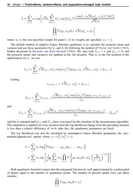
where w i is the user-specified weight for panel i; if no weights are specified, w i = 1.
The default method of adaptive Gauss–Hermite quadrature is to calculate the posterior mean and
variance and use those parameters for ̂µ i and ̂σ i by following the method of Naylor and Smith (1982),
further discussed in Skrondal and Rabe-Hesketh (2004). We start with ̂σ i,0 = 1 and ̂µ i,0 = 0, and
the posterior means and variances are updated in the kth iteration. That is, at the kth iteration of the
optimization for l i , we use
Letting
l i,k ≈
M∑ √
2̂σi,k−1 wm ∗ exp { a ∗ m) 2} g(y it , x it , √ 2̂σ i,k−1 a ∗ m + ̂µ i,k−1 )
m=1
τ i,m,k−1 = √ 2̂σ i,k−1 a ∗ m + ̂µ i,k−1
and
̂σ i,k =
̂µ i,k =
√ M∑
2̂σi,k−1 wm ∗ exp { (a ∗
(τ i,m,k−1 )
m) 2} g(y it , x it , τ i,m,k−1 )
m=1
√ M∑
(τ i,m,k−1 ) 2 2̂σi,k−1 wm ∗ exp { (a ∗ m) 2} g(y it , x it , τ i,m,k−1 )
− (̂µ i,k ) 2
l i,k
m=1
and this is repeated until ̂µ i,k and ̂σ i,k have converged for this iteration of the maximization algorithm.
This adaptation is applied on every iteration until the log-likelihood change from the preceding iteration
is less than a relative difference of 1e–6; after this, the quadrature parameters are fixed.
The log likelihood can also be calculated by nonadaptive Gauss–Hermite quadrature, the intmethod(ghermite)
option, where ρ = σ 2 ν/(σ 2 ν + 1):
L =
≈
n∑
i=1
l i,k
{
}
w i log Pr(y i1 , . . . , y ini |x i1 , . . . , x ini )
[
n∑ 1
w i log √ π
i=1
∑
M n i
wm
∗
m=1 t=1
{
∏
F y it , x it β + a ∗ m
( ) }] 1/2 2ρ
1 − ρ
Both quadrature formulas require that the integrated function be well approximated by a polynomial
of degree equal to the number of quadrature points. The number of periods (panel size) can affect
whether
∏n i
F (y it , x it β + ν i )
t=1