

mixed - Stata
mixed - Stata
mixed - Stata

Create successful ePaper yourself
Turn your PDF publications into a flip-book with our unique Google optimized e-Paper software.
Title<br />
stata.com<br />
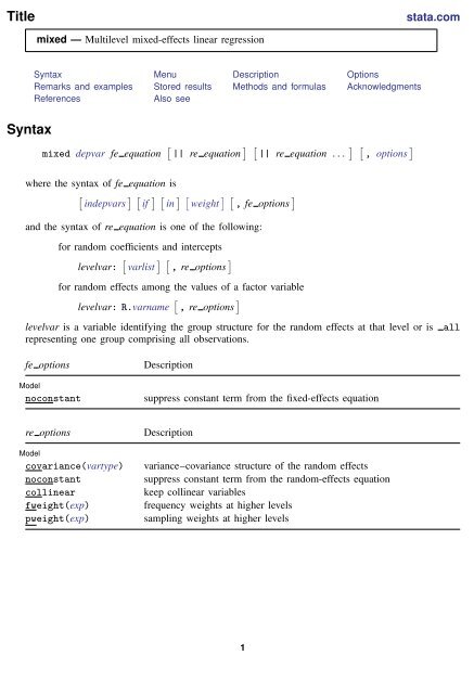
<strong>mixed</strong> — Multilevel <strong>mixed</strong>-effects linear regression<br />
Syntax<br />
Syntax Menu Description Options<br />
Remarks and examples Stored results Methods and formulas Acknowledgments<br />
References<br />
Also see<br />
<strong>mixed</strong> depvar fe equation [ || re equation ] [ || re equation . . . ] [ , options ]<br />
where the syntax of fe equation is<br />
[<br />
indepvars<br />
] [<br />
if<br />
] [<br />
in<br />
] [<br />
weight<br />
] [<br />
, fe options<br />
]<br />
and the syntax of re equation is one of the following:<br />
for random coefficients and intercepts<br />
levelvar: [ varlist ] [ , re options ]<br />
for random effects among the values of a factor variable<br />
levelvar: R.varname [ , re options ]<br />
levelvar is a variable identifying the group structure for the random effects at that level or is<br />
representing one group comprising all observations.<br />
all<br />
fe options<br />
Model<br />
noconstant<br />
Description<br />
suppress constant term from the fixed-effects equation<br />
re options<br />
Model<br />
covariance(vartype)<br />
noconstant<br />
collinear<br />
fweight(exp)<br />
pweight(exp)<br />
Description<br />
variance–covariance structure of the random effects<br />
suppress constant term from the random-effects equation<br />
keep collinear variables<br />
frequency weights at higher levels<br />
sampling weights at higher levels<br />
1
2 <strong>mixed</strong> — Multilevel <strong>mixed</strong>-effects linear regression<br />
options<br />
Model<br />
mle<br />
reml<br />
pwscale(scale method)<br />
residuals(rspec)<br />
SE/Robust<br />
vce(vcetype)<br />
Reporting<br />
level(#)<br />
variance<br />
stddeviations<br />
noretable<br />
nofetable<br />
estmetric<br />
noheader<br />
nogroup<br />
nostderr<br />
nolrtest<br />
display options<br />
EM options<br />
emiterate(#)<br />
emtolerance(#)<br />
emonly<br />
emlog<br />
emdots<br />
Maximization<br />
maximize options<br />
matsqrt<br />
matlog<br />
coeflegend<br />
Description<br />
fit model via maximum likelihood; the default<br />
fit model via restricted maximum likelihood<br />
control scaling of sampling weights in two-level models<br />
structure of residual errors<br />
vcetype may be oim, robust, or cluster clustvar<br />
set confidence level; default is level(95)<br />
show random-effects and residual-error parameter estimates as variances<br />
and covariances; the default<br />
show random-effects and residual-error parameter estimates as standard<br />
deviations<br />
suppress random-effects table<br />
suppress fixed-effects table<br />
show parameter estimates in the estimation metric<br />
suppress output header<br />
suppress table summarizing groups<br />
do not estimate standard errors of random-effects parameters<br />
do not perform likelihood-ratio test comparing with linear regression<br />
control column formats, row spacing, line width, display of omitted<br />
variables and base and empty cells, and factor-variable labeling<br />
number of EM iterations; default is emiterate(20)<br />
EM convergence tolerance; default is emtolerance(1e-10)<br />
fit model exclusively using EM<br />
show EM iteration log<br />
show EM iterations as dots<br />
control the maximization process; seldom used<br />
parameterize variance components using matrix square roots; the default<br />
parameterize variance components using matrix logarithms<br />
display legend instead of statistics
vartype<br />
Description<br />
<strong>mixed</strong> — Multilevel <strong>mixed</strong>-effects linear regression 3<br />
independent one unique variance parameter per random effect, all covariances 0;<br />
the default unless the R. notation is used<br />
exchangeable equal variances for random effects, and one common pairwise<br />
covariance<br />
identity equal variances for random effects, all covariances 0;<br />
the default if the R. notation is used<br />
unstructured all variances and covariances to be distinctly estimated<br />
indepvars may contain factor variables; see [U] 11.4.3 Factor variables.<br />
depvar, indepvars, and varlist may contain time-series operators; see [U] 11.4.4 Time-series varlists.<br />
bootstrap, by, jackknife, mi estimate, rolling, and statsby are allowed; see [U] 11.1.10 Prefix commands.<br />
Weights are not allowed with the bootstrap prefix; see [R] bootstrap.<br />
pweights and fweights are allowed; see [U] 11.1.6 weight.<br />
coeflegend does not appear in the dialog box.<br />
See [U] 20 Estimation and postestimation commands for more capabilities of estimation commands.<br />
Menu<br />
Statistics > Multilevel <strong>mixed</strong>-effects models > Linear regression<br />
Description<br />
<strong>mixed</strong> fits linear <strong>mixed</strong>-effects models. The overall error distribution of the linear <strong>mixed</strong>-effects<br />
model is assumed to be Gaussian, and heteroskedasticity and correlations within lowest-level groups<br />
also may be modeled.<br />
Options<br />
✄<br />
✄<br />
Model<br />
<br />
noconstant suppresses the constant (intercept) term and may be specified for the fixed-effects<br />
equation and for any or all of the random-effects equations.<br />
covariance(vartype), where vartype is<br />
independent | exchangeable | identity | unstructured<br />
specifies the structure of the covariance matrix for the random effects and may be specified for<br />
each random-effects equation. An independent covariance structure allows for a distinct variance<br />
for each random effect within a random-effects equation and assumes that all covariances are 0.<br />
exchangeable structure specifies one common variance for all random effects and one common<br />
pairwise covariance. identity is short for “multiple of the identity”; that is, all variances are<br />
equal and all covariances are 0. unstructured allows for all variances and covariances to be<br />
distinct. If an equation consists of p random-effects terms, the unstructured covariance matrix will<br />
have p(p + 1)/2 unique parameters.<br />
covariance(independent) is the default, except when the R. notation is used, in which<br />
case covariance(identity) is the default and only covariance(identity) and covariance(exchangeable)<br />
are allowed.
4 <strong>mixed</strong> — Multilevel <strong>mixed</strong>-effects linear regression<br />
collinear specifies that <strong>mixed</strong> not omit collinear variables from the random-effects equation.<br />
Usually, there is no reason to leave collinear variables in place; in fact, doing so usually causes<br />
the estimation to fail because of the matrix singularity caused by the collinearity. However, with<br />
certain models (for example, a random-effects model with a full set of contrasts), the variables<br />
may be collinear, yet the model is fully identified because of restrictions on the random-effects<br />
covariance structure. In such cases, using the collinear option allows the estimation to take<br />
place with the random-effects equation intact.<br />
fweight(exp) specifies frequency weights at higher levels in a multilevel model, whereas frequency<br />
weights at the first level (the observation level) are specified in the usual manner, for example,<br />
[fw=fwtvar1]. exp can be any valid <strong>Stata</strong> expression, and you can specify fweight() at levels<br />
two and higher of a multilevel model. For example, in the two-level model<br />
. <strong>mixed</strong> fixed_portion [fw = wt1] || school: . . . , fweight(wt2) . . .<br />
the variable wt1 would hold the first-level (the observation-level) frequency weights, and wt2<br />
would hold the second-level (the school-level) frequency weights.<br />
pweight(exp) specifies sampling weights at higher levels in a multilevel model, whereas sampling<br />
weights at the first level (the observation level) are specified in the usual manner, for example,<br />
[pw=pwtvar1]. exp can be any valid <strong>Stata</strong> expression, and you can specify pweight() at levels<br />
two and higher of a multilevel model. For example, in the two-level model<br />
. <strong>mixed</strong> fixed_portion [pw = wt1] || school: . . . , pweight(wt2) . . .<br />
variable wt1 would hold the first-level (the observation-level) sampling weights, and wt2 would<br />
hold the second-level (the school-level) sampling weights.<br />
See Survey data in Remarks and examples below for more information regarding the use of<br />
sampling weights in multilevel models.<br />
Weighted estimation, whether frequency or sampling, is not supported under restricted maximumlikelihood<br />
estimation (REML).<br />
mle and reml specify the statistical method for fitting the model.<br />
mle, the default, specifies that the model be fit using maximum likelihood (ML).<br />
reml specifies that the model be fit using restricted maximum likelihood (REML), also known as<br />
residual maximum likelihood.<br />
pwscale(scale method), where scale method is<br />
size | effective | gk<br />
controls how sampling weights (if specified) are scaled in two-level models.<br />
scale method size specifies that first-level (observation-level) weights be scaled so that they<br />
sum to the sample size of their corresponding second-level cluster. Second-level sampling<br />
weights are left unchanged.<br />
scale method effective specifies that first-level weights be scaled so that they sum to the<br />
effective sample size of their corresponding second-level cluster. Second-level sampling weights<br />
are left unchanged.<br />
scale method gk specifies the Graubard and Korn (1996) method. Under this method, secondlevel<br />
weights are set to the cluster averages of the products of the weights at both levels, and<br />
first-level weights are then set equal to 1.<br />
pwscale() is supported only with two-level models. See Survey data in Remarks and examples<br />
below for more details on using pwscale().
<strong>mixed</strong> — Multilevel <strong>mixed</strong>-effects linear regression 5<br />
residuals(rspec), where rspec is<br />
restype [ , residual options ]<br />
specifies the structure of the residual errors within the lowest-level groups (the second level of a<br />
multilevel model with the observations comprising the first level) of the linear <strong>mixed</strong> model. For<br />
example, if you are modeling random effects for classes nested within schools, then residuals()<br />
refers to the residual variance–covariance structure of the observations within classes, the lowestlevel<br />
groups.<br />
restype is<br />
independent | exchangeable | ar # | ma # | unstructured |<br />
banded # | toeplitz # | exponential<br />
By default, restype is independent, which means that all residuals are independent and<br />
identically distributed (i.i.d.) Gaussian with one common variance. When combined with<br />
by(varname), independence is still assumed, but you estimate a distinct variance for each<br />
level of varname. Unlike with the structures described below, varname does not need to be<br />
constant within groups.<br />
restype exchangeable estimates two parameters, one common within-group variance and one<br />
common pairwise covariance. When combined with by(varname), these two parameters<br />
are distinctly estimated for each level of varname. Because you are modeling a withingroup<br />
covariance, varname must be constant within lowest-level groups.<br />
restype ar # assumes that within-group errors have an autoregressive (AR) structure of<br />
order #; ar 1 is the default. The t(varname) option is required, where varname is an<br />
integer-valued time variable used to order the observations within groups and to determine<br />
the lags between successive observations. Any nonconsecutive time values will be treated<br />
as gaps. For this structure, # + 1 parameters are estimated (# AR coefficients and one<br />
overall error variance). restype ar may be combined with by(varname), but varname<br />
must be constant within groups.<br />
restype ma # assumes that within-group errors have a moving average (MA) structure of<br />
order #; ma 1 is the default. The t(varname) option is required, where varname is an<br />
integer-valued time variable used to order the observations within groups and to determine<br />
the lags between successive observations. Any nonconsecutive time values will be treated<br />
as gaps. For this structure, # + 1 parameters are estimated (# MA coefficients and one<br />
overall error variance). restype ma may be combined with by(varname), but varname<br />
must be constant within groups.<br />
restype unstructured is the most general structure; it estimates distinct variances for<br />
each within-group error and distinct covariances for each within-group error pair. The<br />
t(varname) option is required, where varname is a nonnegative-integer–valued variable<br />
that identifies the observations within each group. The groups may be unbalanced in that<br />
not all levels of t() need to be observed within every group, but you may not have<br />
repeated t() values within any particular group. When you have p levels of t(), then<br />
p(p + 1)/2 parameters are estimated. restype unstructured may be combined with<br />
by(varname), but varname must be constant within groups.<br />
restype banded # is a special case of unstructured that restricts estimation to the<br />
covariances within the first # off-diagonals and sets the covariances outside this band to<br />
0. The t(varname) option is required, where varname is a nonnegative-integer–valued<br />
variable that identifies the observations within each group. # is an integer between 0 and<br />
p − 1, where p is the number of levels of t(). By default, # is p − 1; that is, all elements
6 <strong>mixed</strong> — Multilevel <strong>mixed</strong>-effects linear regression<br />
✄<br />
of the covariance matrix are estimated. When # is 0, only the diagonal elements of the<br />
covariance matrix are estimated. restype banded may be combined with by(varname),<br />
but varname must be constant within groups.<br />
restype toeplitz # assumes that within-group errors have Toeplitz structure of order #,<br />
for which correlations are constant with respect to time lags less than or equal to #<br />
and are 0 for lags greater than #. The t(varname) option is required, where varname<br />
is an integer-valued time variable used to order the observations within groups and to<br />
determine the lags between successive observations. # is an integer between 1 and the<br />
maximum observed lag (the default). Any nonconsecutive time values will be treated as<br />
gaps. For this structure, # + 1 parameters are estimated (# correlations and one overall<br />
error variance). restype toeplitz may be combined with by(varname), but varname<br />
must be constant within groups.<br />
restype exponential is a generalization of the AR covariance model that allows for unequally<br />
spaced and noninteger time values. The t(varname) option is required, where varname<br />
is real-valued. For the exponential covariance model, the correlation between two errors<br />
is the parameter ρ, raised to a power equal to the absolute value of the difference between<br />
the t() values for those errors. For this structure, two parameters are estimated (the<br />
correlation parameter ρ and one overall error variance). restype exponential may be<br />
combined with by(varname), but varname must be constant within groups.<br />
residual options are by(varname) and t(varname).<br />
✄<br />
by(varname) is for use within the residuals() option and specifies that a set of distinct<br />
residual-error parameters be estimated for each level of varname. In other words, you<br />
use by() to model heteroskedasticity.<br />
t(varname) is for use within the residuals() option to specify a time variable for the<br />
ar, ma, toeplitz, and exponential structures, or to identify the observations when<br />
restype is unstructured or banded.<br />
SE/Robust<br />
<br />
vce(vcetype) specifies the type of standard error reported, which includes types that are derived<br />
from asymptotic theory (oim), that are robust to some kinds of misspecification (robust), and<br />
that allow for intragroup correlation (cluster clustvar); see [R] vce option. If vce(robust) is<br />
specified, robust variances are clustered at the highest level in the multilevel model.<br />
vce(robust) and vce(cluster clustvar) are not supported with REML estimation.<br />
✄ <br />
✄ Reporting<br />
level(#); see [R] estimation options.<br />
variance, the default, displays the random-effects and residual-error parameter estimates as variances<br />
and covariances.<br />
stddeviations displays the random-effects and residual-error parameter estimates as standard<br />
deviations and correlations.<br />
noretable suppresses the random-effects table from the output.<br />
nofetable suppresses the fixed-effects table from the output.<br />
estmetric displays all parameter estimates in the estimation metric. Fixed-effects estimates are<br />
unchanged from those normally displayed, but random-effects parameter estimates are displayed<br />
as log-standard deviations and hyperbolic arctangents of correlations, with equation names that
<strong>mixed</strong> — Multilevel <strong>mixed</strong>-effects linear regression 7<br />
organize them by model level. Residual-variance parameter estimates are also displayed in their<br />
original estimation metric.<br />
noheader suppresses the output header, either at estimation or upon replay.<br />
nogroup suppresses the display of group summary information (number of groups, average group<br />
size, minimum, and maximum) from the output header.<br />
nostderr prevents <strong>mixed</strong> from calculating standard errors for the estimated random-effects parameters,<br />
although standard errors are still provided for the fixed-effects parameters. Specifying this option<br />
will speed up computation times. nostderr is available only when residuals are modeled as<br />
independent with constant variance.<br />
nolrtest prevents <strong>mixed</strong> from fitting a reference linear regression model and using this model to<br />
calculate a likelihood-ratio test comparing the <strong>mixed</strong> model to ordinary regression. This option<br />
may also be specified on replay to suppress this test from the output.<br />
display options: noomitted, vsquish, noemptycells, baselevels, allbaselevels, nofvlabel,<br />
fvwrap(#), fvwrapon(style), cformat(% fmt), pformat(% fmt), sformat(% fmt), and<br />
nolstretch; see [R] estimation options.<br />
✄<br />
✄ <br />
EM options<br />
<br />
These options control the expectation-maximization (EM) iterations that take place before estimation<br />
switches to a gradient-based method. When residuals are modeled as independent with constant<br />
variance, EM will either converge to the solution or bring parameter estimates close to the solution.<br />
For other residual structures or for weighted estimation, EM is used to obtain starting values.<br />
✄<br />
emiterate(#) specifies the number of EM iterations to perform. The default is emiterate(20).<br />
emtolerance(#) specifies the convergence tolerance for the EM algorithm. The default is<br />
emtolerance(1e-10). EM iterations will be halted once the log (restricted) likelihood changes<br />
by a relative amount less than #. At that point, optimization switches to a gradient-based method,<br />
unless emonly is specified, in which case maximization stops.<br />
emonly specifies that the likelihood be maximized exclusively using EM. The advantage of specifying<br />
emonly is that EM iterations are typically much faster than those for gradient-based methods.<br />
The disadvantages are that EM iterations can be slow to converge (if at all) and that EM provides<br />
no facility for estimating standard errors for the random-effects parameters. emonly is available<br />
only with unweighted estimation and when residuals are modeled as independent with constant<br />
variance.<br />
emlog specifies that the EM iteration log be shown. The EM iteration log is, by default, not<br />
displayed unless the emonly option is specified.<br />
emdots specifies that the EM iterations be shown as dots. This option can be convenient because<br />
the EM algorithm may require many iterations to converge.<br />
✄<br />
Maximization<br />
<br />
maximize options: difficult, technique(algorithm spec), iterate(#), [ no ] log, trace,<br />
gradient, showstep, hessian, showtolerance, tolerance(#), ltolerance(#),<br />
nrtolerance(#), and nonrtolerance; see [R] maximize. Those that require special mention<br />
for <strong>mixed</strong> are listed below.<br />
For the technique() option, the default is technique(nr). The bhhh algorithm may not be<br />
specified.<br />
matsqrt (the default), during optimization, parameterizes variance components by using the matrix<br />
square roots of the variance–covariance matrices formed by these components at each model level.
8 <strong>mixed</strong> — Multilevel <strong>mixed</strong>-effects linear regression<br />
matlog, during optimization, parameterizes variance components by using the matrix logarithms of<br />
the variance–covariance matrices formed by these components at each model level.<br />
The matsqrt parameterization ensures that variance–covariance matrices are positive semidefinite,<br />
while matlog ensures matrices that are positive definite. For most problems, the matrix square root<br />
is more stable near the boundary of the parameter space. However, if convergence is problematic,<br />
one option may be to try the alternate matlog parameterization. When convergence is not an issue,<br />
both parameterizations yield equivalent results.<br />
The following option is available with <strong>mixed</strong> but is not shown in the dialog box:<br />
coeflegend; see [R] estimation options.<br />
Remarks and examples<br />
stata.com<br />
Remarks are presented under the following headings:<br />
Introduction<br />
Two-level models<br />
Covariance structures<br />
Likelihood versus restricted likelihood<br />
Three-level models<br />
Blocked-diagonal covariance structures<br />
Heteroskedastic random effects<br />
Heteroskedastic residual errors<br />
Other residual-error structures<br />
Crossed-effects models<br />
Diagnosing convergence problems<br />
Survey data<br />
Introduction<br />
Linear <strong>mixed</strong> models are models containing both fixed effects and random effects. They are a<br />
generalization of linear regression allowing for the inclusion of random deviations (effects) other than<br />
those associated with the overall error term. In matrix notation,<br />
y = Xβ + Zu + ɛ (1)<br />
where y is the n × 1 vector of responses, X is an n × p design/covariate matrix for the fixed effects<br />
β, and Z is the n × q design/covariate matrix for the random effects u. The n × 1 vector of errors<br />
ɛ is assumed to be multivariate normal with mean 0 and variance matrix σ 2 ɛ R.<br />
The fixed portion of (1), Xβ, is analogous to the linear predictor from a standard OLS regression<br />
model with β being the regression coefficients to be estimated. For the random portion of (1), Zu+ɛ,<br />
we assume that u has variance–covariance matrix G and that u is orthogonal to ɛ so that<br />
[ ]<br />
u<br />
Var =<br />
ɛ<br />
[<br />
G 0<br />
]<br />
0 σɛ 2 R<br />
The random effects u are not directly estimated (although they may be predicted), but instead are<br />
characterized by the elements of G, known as variance components, that are estimated along with<br />
the overall residual variance σɛ 2 and the residual-variance parameters that are contained within R.
<strong>mixed</strong> — Multilevel <strong>mixed</strong>-effects linear regression 9<br />
The general forms of the design matrices X and Z allow estimation for a broad class of linear<br />
models: blocked designs, split-plot designs, growth curves, multilevel or hierarchical designs, etc.<br />
They also allow a flexible method of modeling within-cluster correlation. Subjects within the same<br />
cluster can be correlated as a result of a shared random intercept, or through a shared random<br />
slope on (say) age, or both. The general specification of G also provides additional flexibility—the<br />
random intercept and random slope could themselves be modeled as independent, or correlated, or<br />
independent with equal variances, and so forth. The general structure of R also allows for residual<br />
errors to be heteroskedastic and correlated, and allows flexibility in exactly how these characteristics<br />
can be modeled.<br />
Comprehensive treatments of <strong>mixed</strong> models are provided by, among others, Searle, Casella, and<br />
McCulloch (1992); McCulloch, Searle, and Neuhaus (2008); Verbeke and Molenberghs (2000);<br />
Raudenbush and Bryk (2002); Demidenko (2004); and Pinheiro and Bates (2000). In particular,<br />
chapter 2 of Searle, Casella, and McCulloch (1992) provides an excellent history.<br />
The key to fitting <strong>mixed</strong> models lies in estimating the variance components, and for that there exist<br />
many methods. Most of the early literature in <strong>mixed</strong> models dealt with estimating variance components<br />
in ANOVA models. For simple models with balanced data, estimating variance components amounts<br />
to solving a system of equations obtained by setting expected mean-squares expressions equal to their<br />
observed counterparts. Much of the work in extending the ANOVA method to unbalanced data for<br />
general ANOVA designs is due to Henderson (1953).<br />
The ANOVA method, however, has its shortcomings. Among these is a lack of uniqueness in that<br />
alternative, unbiased estimates of variance components could be derived using other quadratic forms<br />
of the data in place of observed mean squares (Searle, Casella, and McCulloch 1992, 38–39). As a<br />
result, ANOVA methods gave way to more modern methods, such as minimum norm quadratic unbiased<br />
estimation (MINQUE) and minimum variance quadratic unbiased estimation (MIVQUE); see Rao (1973)<br />
for MINQUE and LaMotte (1973) for MIVQUE. Both methods involve finding optimal quadratic forms<br />
of the data that are unbiased for the variance components.<br />
The most popular methods, however, are ML and REML, and these are the two methods that are<br />
supported by <strong>mixed</strong>. The ML estimates are based on the usual application of likelihood theory, given<br />
the distributional assumptions of the model. The basic idea behind REML (Thompson 1962) is that<br />
you can form a set of linear contrasts of the response that do not depend on the fixed effects β, but<br />
instead depend only on the variance components to be estimated. You then apply ML methods by<br />
using the distribution of the linear contrasts to form the likelihood.<br />
Returning to (1): in clustered-data situations, it is convenient not to consider all n observations at<br />
once but instead to organize the <strong>mixed</strong> model as a series of M independent groups (or clusters)<br />
y j = X j β + Z j u j + ɛ j (2)<br />
for j = 1, . . . , M, with cluster j consisting of n j observations. The response y j comprises the rows<br />
of y corresponding with the jth cluster, with X j and ɛ j defined analogously. The random effects u j<br />
can now be thought of as M realizations of a q × 1 vector that is normally distributed with mean 0<br />
and q × q variance matrix Σ. The matrix Z i is the n j × q design matrix for the jth cluster random<br />
effects. Relating this to (1), note that<br />
⎡<br />
⎤<br />
Z 1 0 · · · 0<br />
0 Z<br />
Z = ⎢ 2 · · · 0<br />
⎣<br />
.<br />
.<br />
. ..<br />
. ..<br />
0 0 0 Z M<br />
⎥<br />
⎦ ;<br />
⎡ ⎤<br />
u 1<br />
u = ⎣ . ⎦<br />
. ; G = I M ⊗ Σ; R = I M ⊗ Λ (3)<br />
u M<br />
The <strong>mixed</strong>-model formulation (2) is from Laird and Ware (1982) and offers two key advantages.<br />
First, it makes specifications of random-effects terms easier. If the clusters are schools, you can
10 <strong>mixed</strong> — Multilevel <strong>mixed</strong>-effects linear regression<br />
simply specify a random effect at the school level, as opposed to thinking of what a school-level<br />
random effect would mean when all the data are considered as a whole (if it helps, think Kronecker<br />
products). Second, representing a <strong>mixed</strong>-model with (2) generalizes easily to more than one set of<br />
random effects. For example, if classes are nested within schools, then (2) can be generalized to allow<br />
random effects at both the school and the class-within-school levels. This we demonstrate later.<br />
In the sections that follow, we assume that residuals are independent with constant variance; that<br />
is, in (3) we treat Λ equal to the identity matrix and limit ourselves to estimating one overall residual<br />
variance, σɛ 2 . Beginning in Heteroskedastic residual errors, we relax this assumption.<br />
Two-level models<br />
We begin with a simple application of (2) as a two-level model, because a one-level linear model,<br />
by our terminology, is just standard OLS regression.<br />
Example 1<br />
Consider a longitudinal dataset, used by both Ruppert, Wand, and Carroll (2003) and Diggle<br />
et al. (2002), consisting of weight measurements of 48 pigs on 9 successive weeks. Pigs are<br />
identified by the variable id. Below is a plot of the growth curves for the first 10 pigs.<br />
. use http://www.stata-press.com/data/r13/pig<br />
(Longitudinal analysis of pig weights)<br />
. twoway connected weight week if id
<strong>mixed</strong> — Multilevel <strong>mixed</strong>-effects linear regression 11<br />
. <strong>mixed</strong> weight week || id:<br />
Performing EM optimization:<br />
Performing gradient-based optimization:<br />
Iteration 0: log likelihood = -1014.9268<br />
Iteration 1: log likelihood = -1014.9268<br />
Computing standard errors:<br />
Mixed-effects ML regression Number of obs = 432<br />
Group variable: id Number of groups = 48<br />
Obs per group: min = 9<br />
avg = 9.0<br />
max = 9<br />
Wald chi2(1) = 25337.49<br />
Log likelihood = -1014.9268 Prob > chi2 = 0.0000<br />
weight Coef. Std. Err. z P>|z| [95% Conf. Interval]<br />
week 6.209896 .0390124 159.18 0.000 6.133433 6.286359<br />
_cons 19.35561 .5974059 32.40 0.000 18.18472 20.52651<br />
Random-effects Parameters Estimate Std. Err. [95% Conf. Interval]<br />
id: Identity<br />
var(_cons) 14.81751 3.124226 9.801716 22.40002<br />
Notes:<br />
var(Residual) 4.383264 .3163348 3.805112 5.04926<br />
LR test vs. linear regression: chibar2(01) = 472.65 Prob >= chibar2 = 0.0000<br />
1. By typing weight week, we specified the response, weight, and the fixed portion of the model<br />
in the same way that we would if we were using regress or any other estimation command. Our<br />
fixed effects are a coefficient on week and a constant term.<br />
2. When we added || id:, we specified random effects at the level identified by the group variable<br />
id, that is, the pig level (level two). Because we wanted only a random intercept, that is all we<br />
had to type.<br />
3. The estimation log consists of three parts:<br />
a. A set of EM iterations used to refine starting values. By default, the iterations themselves are<br />
not displayed, but you can display them with the emlog option.<br />
b. A set of gradient-based iterations. By default, these are Newton–Raphson iterations, but other<br />
methods are available by specifying the appropriate maximize options; see [R] maximize.<br />
c. The message “Computing standard errors”. This is just to inform you that <strong>mixed</strong> has finished<br />
its iterative maximization and is now reparameterizing from a matrix-based parameterization<br />
(see Methods and formulas) to the natural metric of variance components and their estimated<br />
standard errors.<br />
4. The output title, “Mixed-effects ML regression”, informs us that our model was fit using ML, the<br />
default. For REML estimates, use the reml option.<br />
Because this model is a simple random-intercept model fit by ML, it would be equivalent to using<br />
xtreg with its mle option.<br />
5. The first estimation table reports the fixed effects. We estimate β 0 = 19.36 and β 1 = 6.21.
12 <strong>mixed</strong> — Multilevel <strong>mixed</strong>-effects linear regression<br />
6. The second estimation table shows the estimated variance components. The first section of the<br />
table is labeled id: Identity, meaning that these are random effects at the id (pig) level and that<br />
their variance–covariance matrix is a multiple of the identity matrix; that is, Σ = σuI. 2 Because<br />
we have only one random effect at this level, <strong>mixed</strong> knew that Identity is the only possible<br />
covariance structure. In any case, the variance of the level-two errors, σu 2 , is estimated as 14.82<br />
with standard error 3.12.<br />
7. The row labeled var(Residual) displays the estimated variance of the overall error term; that<br />
is, ̂σ 2 ɛ = 4.38. This is the variance of the level-one errors, that is, the residuals.<br />
8. Finally, a likelihood-ratio test comparing the model with one-level ordinary linear regression, model<br />
(4) without u j , is provided and is highly significant for these data.<br />
We now store our estimates for later use:<br />
. estimates store randint<br />
Example 2<br />
Extending (4) to allow for a random slope on week yields the model<br />
and we fit this with <strong>mixed</strong>:<br />
. <strong>mixed</strong> weight week || id: week<br />
Performing EM optimization:<br />
weight ij = β 0 + β 1 week ij + u 0j + u 1j week ij + ɛ ij (5)<br />
Performing gradient-based optimization:<br />
Iteration 0: log likelihood = -869.03825<br />
Iteration 1: log likelihood = -869.03825<br />
Computing standard errors:<br />
Mixed-effects ML regression Number of obs = 432<br />
Group variable: id Number of groups = 48<br />
Obs per group: min = 9<br />
avg = 9.0<br />
max = 9<br />
Wald chi2(1) = 4689.51<br />
Log likelihood = -869.03825 Prob > chi2 = 0.0000<br />
weight Coef. Std. Err. z P>|z| [95% Conf. Interval]<br />
week 6.209896 .0906819 68.48 0.000 6.032163 6.387629<br />
_cons 19.35561 .3979159 48.64 0.000 18.57571 20.13551<br />
Random-effects Parameters Estimate Std. Err. [95% Conf. Interval]<br />
id: Independent<br />
var(week) .3680668 .0801181 .2402389 .5639103<br />
var(_cons) 6.756364 1.543503 4.317721 10.57235<br />
var(Residual) 1.598811 .1233988 1.374358 1.85992<br />
LR test vs. linear regression: chi2(2) = 764.42 Prob > chi2 = 0.0000<br />
Note: LR test is conservative and provided only for reference.<br />
. estimates store randslope
<strong>mixed</strong> — Multilevel <strong>mixed</strong>-effects linear regression 13<br />
Because we did not specify a covariance structure for the random effects (u 0j , u 1j ) ′ , <strong>mixed</strong> used<br />
the default Independent structure; that is,<br />
[ ] [ ]<br />
u0j σ<br />
2<br />
Σ = Var = u0 0<br />
u 1j 0 σu1<br />
2<br />
with ̂σ u0 2 = 6.76 and ̂σ u1 2 = 0.37. Our point estimates of the fixed effects are essentially identical to<br />
those from model (4), but note that this does not hold generally. Given the 95% confidence interval<br />
for ̂σ u1 2 , it would seem that the random slope is significant, and we can use lrtest and our two<br />
stored estimation results to verify this fact:<br />
. lrtest randslope randint<br />
Likelihood-ratio test LR chi2(1) = 291.78<br />
(Assumption: randint nested in randslope) Prob > chi2 = 0.0000<br />
Note: The reported degrees of freedom assumes the null hypothesis is not on<br />
the boundary of the parameter space. If this is not true, then the<br />
reported test is conservative.<br />
The near-zero significance level favors the model that allows for a random pig-specific regression<br />
line over the model that allows only for a pig-specific shift.<br />
(6)<br />
Covariance structures<br />
In example 2, we fit a model with the default Independent covariance given in (6). Within any<br />
random-effects level specification, we can override this default by specifying an alternative covariance<br />
structure via the covariance() option.<br />
Example 3<br />
We generalize (6) to allow u 0j and u 1j to be correlated; that is,<br />
[ ] [ ]<br />
u0j σ<br />
2<br />
Σ = Var = u0 σ 01<br />
u 1j σ 01 σu1<br />
2
14 <strong>mixed</strong> — Multilevel <strong>mixed</strong>-effects linear regression<br />
. <strong>mixed</strong> weight week || id: week, covariance(unstructured)<br />
Performing EM optimization:<br />
Performing gradient-based optimization:<br />
Iteration 0: log likelihood = -868.96185<br />
Iteration 1: log likelihood = -868.96185<br />
Computing standard errors:<br />
Mixed-effects ML regression Number of obs = 432<br />
Group variable: id Number of groups = 48<br />
Obs per group: min = 9<br />
avg = 9.0<br />
max = 9<br />
Wald chi2(1) = 4649.17<br />
Log likelihood = -868.96185 Prob > chi2 = 0.0000<br />
weight Coef. Std. Err. z P>|z| [95% Conf. Interval]<br />
week 6.209896 .0910745 68.18 0.000 6.031393 6.388399<br />
_cons 19.35561 .3996387 48.43 0.000 18.57234 20.13889<br />
Random-effects Parameters Estimate Std. Err. [95% Conf. Interval]<br />
id: Unstructured<br />
var(week) .3715251 .0812958 .2419532 .570486<br />
var(_cons) 6.823363 1.566194 4.351297 10.69986<br />
cov(week,_cons) -.0984378 .2545767 -.5973991 .4005234<br />
var(Residual) 1.596829 .123198 1.372735 1.857505<br />
LR test vs. linear regression: chi2(3) = 764.58 Prob > chi2 = 0.0000<br />
Note: LR test is conservative and provided only for reference.<br />
But we do not find the correlation to be at all significant.<br />
. lrtest . randslope<br />
Likelihood-ratio test LR chi2(1) = 0.15<br />
(Assumption: randslope nested in .) Prob > chi2 = 0.6959<br />
Instead, we could have also specified covariance(identity), restricting u 0j and u 1j to not<br />
only be independent but also to have common variance, or we could have specified covariance(exchangeable),<br />
which imposes a common variance but allows for a nonzero correlation.<br />
Likelihood versus restricted likelihood<br />
Thus far, all our examples have used ML to estimate variance components. We could have just as<br />
easily asked for REML estimates. Refitting the model in example 2 by REML, we get
<strong>mixed</strong> — Multilevel <strong>mixed</strong>-effects linear regression 15<br />
. <strong>mixed</strong> weight week || id: week, reml<br />
Performing EM optimization:<br />
Performing gradient-based optimization:<br />
Iteration 0: log restricted-likelihood = -870.51473<br />
Iteration 1: log restricted-likelihood = -870.51473<br />
Computing standard errors:<br />
Mixed-effects REML regression Number of obs = 432<br />
Group variable: id Number of groups = 48<br />
Obs per group: min = 9<br />
avg = 9.0<br />
max = 9<br />
Wald chi2(1) = 4592.10<br />
Log restricted-likelihood = -870.51473 Prob > chi2 = 0.0000<br />
weight Coef. Std. Err. z P>|z| [95% Conf. Interval]<br />
week 6.209896 .0916387 67.77 0.000 6.030287 6.389504<br />
_cons 19.35561 .4021144 48.13 0.000 18.56748 20.14374<br />
Random-effects Parameters Estimate Std. Err. [95% Conf. Interval]<br />
id: Independent<br />
var(week) .3764405 .0827027 .2447317 .5790317<br />
var(_cons) 6.917604 1.593247 4.404624 10.86432<br />
var(Residual) 1.598784 .1234011 1.374328 1.859898<br />
LR test vs. linear regression: chi2(2) = 765.92 Prob > chi2 = 0.0000<br />
Note: LR test is conservative and provided only for reference.<br />
Although ML estimators are based on the usual likelihood theory, the idea behind REML is to<br />
transform the response into a set of linear contrasts whose distribution is free of the fixed effects β.<br />
The restricted likelihood is then formed by considering the distribution of the linear contrasts. Not<br />
only does this make the maximization problem free of β, it also incorporates the degrees of freedom<br />
used to estimate β into the estimation of the variance components. This follows because, by necessity,<br />
the rank of the linear contrasts must be less than the number of observations.<br />
As a simple example, consider a constant-only regression where y i ∼ N(µ, σ 2 ) for i = 1, . . . , n.<br />
The ML estimate of σ 2 can be derived theoretically as the n-divided sample variance. The REML<br />
estimate can be derived by considering the first n − 1 error contrasts, y i − y, whose joint distribution<br />
is free of µ. Applying maximum likelihood to this distribution results in an estimate of σ 2 , that is,<br />
the (n − 1)-divided sample variance, which is unbiased for σ 2 .<br />
The unbiasedness property of REML extends to all <strong>mixed</strong> models when the data are balanced, and<br />
thus REML would seem the clear choice in balanced-data problems, although in large samples the<br />
difference between ML and REML is negligible. One disadvantage of REML is that likelihood-ratio (LR)<br />
tests based on REML are inappropriate for comparing models with different fixed-effects specifications.<br />
ML is appropriate for such LR tests and has the advantage of being easy to explain and being the<br />
method of choice for other estimators.<br />
Another factor to consider is that ML estimation under <strong>mixed</strong> is more feature-rich, allowing for<br />
weighted estimation and robust variance–covariance matrices, features not supported under REML. In<br />
the end, which method to use should be based both on your needs and on personal taste.
16 <strong>mixed</strong> — Multilevel <strong>mixed</strong>-effects linear regression<br />
Examining the REML output, we find that the estimates of the variance components are slightly<br />
larger than the ML estimates. This is typical, because ML estimates, which do not incorporate the<br />
degrees of freedom used to estimate the fixed effects, tend to be biased downward.<br />
Three-level models<br />
The clustered-data representation of the <strong>mixed</strong> model given in (2) can be extended to two nested<br />
levels of clustering, creating a three-level model once the observations are considered. Formally,<br />
y jk = X jk β + Z (3)<br />
jk u(3) k<br />
+ Z (2)<br />
jk u(2) jk + ɛ jk (7)<br />
for i = 1, . . . , n jk first-level observations nested within j = 1, . . . , M k second-level groups, which<br />
are nested within k = 1, . . . , M third-level groups. Group j, k consists of n jk observations, so y jk ,<br />
X jk , and ɛ jk each have row dimension n jk . Z (3)<br />
jk<br />
is the n jk × q 3 design matrix for the third-level<br />
random effects u (3)<br />
k<br />
, and Z(2)<br />
jk is the n jk × q 2 design matrix for the second-level random effects u (2)<br />
jk .<br />
Furthermore, assume that<br />
u (3)<br />
k<br />
∼ N(0, Σ 3 ); u (2)<br />
jk ∼ N(0, Σ 2); ɛ jk ∼ N(0, σ 2 ɛ I)<br />
and that u (3)<br />
k<br />
, u(2) jk , and ɛ jk are independent.<br />
Fitting a three-level model requires you to specify two random-effects equations: one for level<br />
three and then one for level two. The variable list for the first equation represents Z (3)<br />
jk<br />
second equation represents Z (2)<br />
jk<br />
; that is, you specify the levels top to bottom in <strong>mixed</strong>.<br />
Example 4<br />
and for the<br />
Baltagi, Song, and Jung (2001) estimate a Cobb–Douglas production function examining the<br />
productivity of public capital in each state’s private output. Originally provided by Munnell (1990),<br />
the data were recorded over 1970–1986 for 48 states grouped into nine regions.
<strong>mixed</strong> — Multilevel <strong>mixed</strong>-effects linear regression 17<br />
. use http://www.stata-press.com/data/r13/productivity<br />
(Public Capital Productivity)<br />
. describe<br />
Contains data from http://www.stata-press.com/data/r13/productivity.dta<br />
obs: 816 Public Capital Productivity<br />
vars: 11 29 Mar 2013 10:57<br />
size: 29,376 (_dta has notes)<br />
storage display value<br />
variable name type format label variable label<br />
state byte %9.0g states 1-48<br />
region byte %9.0g regions 1-9<br />
year int %9.0g years 1970-1986<br />
public float %9.0g public capital stock<br />
hwy float %9.0g log(highway component of public)<br />
water float %9.0g log(water component of public)<br />
other float %9.0g log(bldg/other component of<br />
public)<br />
private float %9.0g log(private capital stock)<br />
gsp float %9.0g log(gross state product)<br />
emp float %9.0g log(non-agriculture payrolls)<br />
unemp float %9.0g state unemployment rate<br />
Sorted by:<br />
Because the states are nested within regions, we fit a three-level <strong>mixed</strong> model with random intercepts<br />
at both the region and the state-within-region levels. That is, we use (7) with both Z (3)<br />
jk<br />
and Z(2)<br />
jk<br />
set<br />
to the n jk × 1 column of ones, and Σ 3 = σ3 2 and Σ 2 = σ2 2 are both scalars.<br />
. <strong>mixed</strong> gsp private emp hwy water other unemp || region: || state:<br />
(output omitted )<br />
Mixed-effects ML regression Number of obs = 816<br />
No. of Observations per Group<br />
Group Variable Groups Minimum Average Maximum<br />
region 9 51 90.7 136<br />
state 48 17 17.0 17<br />
Wald chi2(6) = 18829.06<br />
Log likelihood = 1430.5017 Prob > chi2 = 0.0000<br />
gsp Coef. Std. Err. z P>|z| [95% Conf. Interval]<br />
private .2671484 .0212591 12.57 0.000 .2254814 .3088154<br />
emp .754072 .0261868 28.80 0.000 .7027468 .8053973<br />
hwy .0709767 .023041 3.08 0.002 .0258172 .1161363<br />
water .0761187 .0139248 5.47 0.000 .0488266 .1034109<br />
other -.0999955 .0169366 -5.90 0.000 -.1331906 -.0668004<br />
unemp -.0058983 .0009031 -6.53 0.000 -.0076684 -.0041282<br />
_cons 2.128823 .1543854 13.79 0.000 1.826233 2.431413
18 <strong>mixed</strong> — Multilevel <strong>mixed</strong>-effects linear regression<br />
Random-effects Parameters Estimate Std. Err. [95% Conf. Interval]<br />
region: Identity<br />
state: Identity<br />
var(_cons) .0014506 .0012995 .0002506 .0083957<br />
var(_cons) .0062757 .0014871 .0039442 .0099855<br />
Notes:<br />
var(Residual) .0013461 .0000689 .0012176 .0014882<br />
LR test vs. linear regression: chi2(2) = 1154.73 Prob > chi2 = 0.0000<br />
Note: LR test is conservative and provided only for reference.<br />
1. Our model now has two random-effects equations, separated by ||. The first is a random intercept<br />
(constant only) at the region level (level three), and the second is a random intercept at the state<br />
level (level two). The order in which these are specified (from left to right) is significant—<strong>mixed</strong><br />
assumes that state is nested within region.<br />
2. The information on groups is now displayed as a table, with one row for each grouping. You can<br />
suppress this table with the nogroup or the noheader option, which will suppress the rest of the<br />
header, as well.<br />
3. The variance-component estimates are now organized and labeled according to level.<br />
After adjusting for the nested-level error structure, we find that the highway and water components<br />
of public capital had significant positive effects on private output, whereas the other public buildings<br />
component had a negative effect.<br />
Technical note<br />
In the previous example, the states are coded 1–48 and are nested within nine regions. <strong>mixed</strong><br />
treated the states as nested within regions, regardless of whether the codes for each state were unique<br />
between regions. That is, even if codes for states were duplicated between regions, <strong>mixed</strong> would<br />
have enforced the nesting and produced the same results.<br />
The group information at the top of the <strong>mixed</strong> output and that produced by the postestimation<br />
command estat group (see [ME] <strong>mixed</strong> postestimation) take the nesting into account. The statistics<br />
are thus not necessarily what you would get if you instead tabulated each group variable individually.<br />
Model (7) extends in a straightforward manner to more than three levels, as does the specification<br />
of such models in <strong>mixed</strong>.<br />
Blocked-diagonal covariance structures<br />
Covariance matrices of random effects within an equation can be modeled either as a multiple of<br />
the identity matrix, as diagonal (that is, Independent), as exchangeable, or as general symmetric<br />
(Unstructured). These may also be combined to produce more complex block-diagonal covariance<br />
structures, effectively placing constraints on the variance components.
<strong>mixed</strong> — Multilevel <strong>mixed</strong>-effects linear regression 19<br />
Example 5<br />
Returning to our productivity data, we now add random coefficients on hwy and unemp at the<br />
region level. This only slightly changes the estimates of the fixed effects, so we focus our attention<br />
on the variance components:<br />
. <strong>mixed</strong> gsp private emp hwy water other unemp || region: hwy unemp || state:,<br />
> nolog nogroup nofetable<br />
Mixed-effects ML regression Number of obs = 816<br />
Wald chi2(6) = 17137.94<br />
Log likelihood = 1447.6787 Prob > chi2 = 0.0000<br />
Random-effects Parameters Estimate Std. Err. [95% Conf. Interval]<br />
region: Independent<br />
var(hwy) .0000209 .0001103 6.71e-10 .650695<br />
var(unemp) .0000238 .0000135 7.84e-06 .0000722<br />
var(_cons) .0030349 .0086684 .0000112 .8191296<br />
state: Identity<br />
var(_cons) .0063658 .0015611 .0039365 .0102943<br />
var(Residual) .0012469 .0000643 .001127 .0013795<br />
LR test vs. linear regression: chi2(4) = 1189.08 Prob > chi2 = 0.0000<br />
Note: LR test is conservative and provided only for reference.<br />
. estimates store prodrc<br />
This model is the same as that fit in example 4 except that Z (3)<br />
jk<br />
is now the n jk × 3 matrix with<br />
columns determined by the values of hwy, unemp, and an intercept term (one), in that order, and<br />
(because we used the default Independent structure) Σ 3 is<br />
Σ 3 =<br />
(<br />
hwy unemp cons<br />
σa 2 )<br />
0 0<br />
0 σb 2 0<br />
0 0 σc<br />
2<br />
The random-effects specification at the state level remains unchanged; that is, Σ 2 is still treated as<br />
the scalar variance of the random intercepts at the state level.<br />
An LR test comparing this model with that from example 4 favors the inclusion of the two random<br />
coefficients, a fact we leave to the interested reader to verify.<br />
The estimated variance components, upon examination, reveal that the variances of the random<br />
coefficients on hwy and unemp could be treated as equal. That is,<br />
Σ 3 =<br />
(<br />
hwy unemp cons<br />
σa 2 )<br />
0 0<br />
0 σa 2 0<br />
0 0 σc<br />
2<br />
looks plausible. We can impose this equality constraint by treating Σ 3 as block diagonal: the first<br />
block is a 2 × 2 multiple of the identity matrix, that is, σ 2 aI 2 ; the second is a scalar, equivalently, a<br />
1 × 1 multiple of the identity.
20 <strong>mixed</strong> — Multilevel <strong>mixed</strong>-effects linear regression<br />
We construct block-diagonal covariances by repeating level specifications:<br />
. <strong>mixed</strong> gsp private emp hwy water other unemp || region: hwy unemp,<br />
> cov(identity) || region: || state:, nolog nogroup nofetable<br />
Mixed-effects ML regression Number of obs = 816<br />
Wald chi2(6) = 17136.65<br />
Log likelihood = 1447.6784 Prob > chi2 = 0.0000<br />
Random-effects Parameters Estimate Std. Err. [95% Conf. Interval]<br />
region: Identity<br />
var(hwy unemp) .0000238 .0000134 7.89e-06 .0000719<br />
region: Identity<br />
state: Identity<br />
var(_cons) .0028191 .0030429 .0003399 .023383<br />
var(_cons) .006358 .0015309 .0039661 .0101925<br />
var(Residual) .0012469 .0000643 .001127 .0013795<br />
LR test vs. linear regression: chi2(3) = 1189.08 Prob > chi2 = 0.0000<br />
Note: LR test is conservative and provided only for reference.<br />
We specified two equations for the region level: the first for the random coefficients on hwy and<br />
unemp with covariance set to Identity and the second for the random intercept cons, whose<br />
covariance defaults to Identity because it is of dimension 1. <strong>mixed</strong> labeled the estimate of σa 2 as<br />
var(hwy unemp) to designate that it is common to the random coefficients on both hwy and unemp.<br />
An LR test shows that the constrained model fits equally well.<br />
. lrtest . prodrc<br />
Likelihood-ratio test LR chi2(1) = 0.00<br />
(Assumption: . nested in prodrc) Prob > chi2 = 0.9784<br />
Note: The reported degrees of freedom assumes the null hypothesis is not on<br />
the boundary of the parameter space. If this is not true, then the<br />
reported test is conservative.<br />
Because the null hypothesis for this test is one of equality (H 0 : σa 2 = σb 2 ), it is not on the<br />
boundary of the parameter space. As such, we can take the reported significance as precise rather<br />
than a conservative estimate.<br />
You can repeat level specifications as often as you like, defining successive blocks of a blockdiagonal<br />
covariance matrix. However, repeated-level equations must be listed consecutively; otherwise,<br />
<strong>mixed</strong> will give an error.<br />
Technical note<br />
In the previous estimation output, there was no constant term included in the first region equation,<br />
even though we did not use the noconstant option. When you specify repeated-level equations,<br />
<strong>mixed</strong> knows not to put constant terms in each equation because such a model would be unidentified.<br />
By default, it places the constant in the last repeated-level equation, but you can use noconstant<br />
creatively to override this.<br />
Linear <strong>mixed</strong>-effects models can also be fit using meglm with the default gaussian family. meglm<br />
provides two more covariance structures through which you can impose constraints on variance<br />
components; see [ME] meglm for details.
<strong>mixed</strong> — Multilevel <strong>mixed</strong>-effects linear regression 21<br />
Heteroskedastic random effects<br />
Blocked-diagonal covariance structures and repeated-level specifications of random effects can also<br />
be used to model heteroskedasticity among random effects at a given level.<br />
Example 6<br />
Following Rabe-Hesketh and Skrondal (2012, sec. 7.2), we analyze data from Asian children in<br />
a British community who were weighed up to four times, roughly between the ages of 6 weeks and<br />
27 months. The dataset is a random sample of data previously analyzed by Goldstein (1986) and<br />
Prosser, Rasbash, and Goldstein (1991).<br />
. use http://www.stata-press.com/data/r13/childweight<br />
(Weight data on Asian children)<br />
. describe<br />
Contains data from http://www.stata-press.com/data/r13/childweight.dta<br />
obs: 198 Weight data on Asian children<br />
vars: 5 23 May 2013 15:12<br />
size: 3,168 (_dta has notes)<br />
storage display value<br />
variable name type format label variable label<br />
id int %8.0g child identifier<br />
age float %8.0g age in years<br />
weight float %8.0g weight in Kg<br />
brthwt int %8.0g Birth weight in g<br />
girl float %9.0g bg gender<br />
Sorted by: id age<br />
. graph twoway (line weight age, connect(ascending)), by(girl)<br />
> xtitle(Age in years) ytitle(Weight in kg)<br />
boy<br />
girl<br />
Weight in kg<br />
5 10 15 20<br />
0 1 2 3 0 1 2 3<br />
Graphs by gender<br />
Age in years<br />
Ignoring gender effects for the moment, we begin with the following model for the ith measurement<br />
on the jth child:<br />
weight ij = β 0 + β 1 age ij + β 2 age 2 ij + u j0 + u j1 age ij + ɛ ij
22 <strong>mixed</strong> — Multilevel <strong>mixed</strong>-effects linear regression<br />
This models overall mean growth as quadratic in age and allows for two child-specific random<br />
effects: a random intercept u j0 , which represents each child’s vertical shift from the overall mean<br />
(β 0 ), and a random age slope u j1 , which represents each child’s deviation in linear growth rate from<br />
the overall mean linear growth rate (β 1 ). For simplicity, we do not consider child-specific changes in<br />
the quadratic component of growth.<br />
. <strong>mixed</strong> weight age c.age#c.age || id: age, nolog<br />
Mixed-effects ML regression Number of obs = 198<br />
Group variable: id Number of groups = 68<br />
Obs per group: min = 1<br />
avg = 2.9<br />
max = 5<br />
Wald chi2(2) = 1863.46<br />
Log likelihood = -258.51915 Prob > chi2 = 0.0000<br />
weight Coef. Std. Err. z P>|z| [95% Conf. Interval]<br />
age 7.693701 .2381076 32.31 0.000 7.227019 8.160384<br />
c.age#c.age -1.654542 .0874987 -18.91 0.000 -1.826037 -1.483048<br />
_cons 3.497628 .1416914 24.68 0.000 3.219918 3.775338<br />
Random-effects Parameters Estimate Std. Err. [95% Conf. Interval]<br />
id: Independent<br />
var(age) .2987207 .0827569 .1735603 .5141388<br />
var(_cons) .5023857 .141263 .2895294 .8717297<br />
var(Residual) .3092897 .0474887 .2289133 .417888<br />
LR test vs. linear regression: chi2(2) = 114.70 Prob > chi2 = 0.0000<br />
Note: LR test is conservative and provided only for reference.<br />
Because there is no reason to believe that the random effects are uncorrelated, it is always a good<br />
idea to first fit a model with the covariance(unstructured) option. We do not include the output<br />
for such a model because for these data the correlation between random effects is not significant;<br />
however, we did check this before reverting to <strong>mixed</strong>’s default Independent structure.<br />
Next we introduce gender effects into the fixed portion of the model by including a main gender<br />
effect and a gender–age interaction for overall mean growth:
<strong>mixed</strong> — Multilevel <strong>mixed</strong>-effects linear regression 23<br />
. <strong>mixed</strong> weight i.girl i.girl#c.age c.age#c.age || id: age, nolog<br />
Mixed-effects ML regression Number of obs = 198<br />
Group variable: id Number of groups = 68<br />
Obs per group: min = 1<br />
avg = 2.9<br />
max = 5<br />
Wald chi2(4) = 1942.30<br />
Log likelihood = -253.182 Prob > chi2 = 0.0000<br />
weight Coef. Std. Err. z P>|z| [95% Conf. Interval]<br />
girl<br />
girl -.5104676 .2145529 -2.38 0.017 -.9309835 -.0899516<br />
girl#c.age<br />
boy 7.806765 .2524583 30.92 0.000 7.311956 8.301574<br />
girl 7.577296 .2531318 29.93 0.000 7.081166 8.073425<br />
c.age#c.age -1.654323 .0871752 -18.98 0.000 -1.825183 -1.483463<br />
_cons 3.754275 .1726404 21.75 0.000 3.415906 4.092644<br />
Random-effects Parameters Estimate Std. Err. [95% Conf. Interval]<br />
id: Independent<br />
var(age) .2772846 .0769233 .1609861 .4775987<br />
var(_cons) .4076892 .12386 .2247635 .7394906<br />
var(Residual) .3131704 .047684 .2323672 .422072<br />
LR test vs. linear regression: chi2(2) = 104.39 Prob > chi2 = 0.0000<br />
Note: LR test is conservative and provided only for reference.<br />
. estimates store homoskedastic<br />
The main gender effect is significant at the 5% level, but the gender–age interaction is not:<br />
. test 0.girl#c.age = 1.girl#c.age<br />
( 1) [weight]0b.girl#c.age - [weight]1.girl#c.age = 0<br />
chi2( 1) = 1.66<br />
Prob > chi2 = 0.1978<br />
On average, boys are heavier than girls, but their average linear growth rates are not significantly<br />
different.<br />
In the above model, we introduced a gender effect on average growth, but we still assumed that the<br />
variability in child-specific deviations from this average was the same for boys and girls. To check<br />
this assumption, we introduce gender into the random component of the model. Because support<br />
for factor-variable notation is limited in specifications of random effects (see Crossed-effects models<br />
below), we need to generate the interactions ourselves.
24 <strong>mixed</strong> — Multilevel <strong>mixed</strong>-effects linear regression<br />
. gen boy = !girl<br />
. gen boyXage = boy*age<br />
. gen girlXage = girl*age<br />
. <strong>mixed</strong> weight i.girl i.girl#c.age c.age#c.age || id: boy boyXage, noconstant<br />
> || id: girl girlXage, noconstant nolog nofetable<br />
Mixed-effects ML regression Number of obs = 198<br />
Group variable: id Number of groups = 68<br />
Obs per group: min = 1<br />
avg = 2.9<br />
max = 5<br />
Wald chi2(4) = 2358.11<br />
Log likelihood = -248.94752 Prob > chi2 = 0.0000<br />
Random-effects Parameters Estimate Std. Err. [95% Conf. Interval]<br />
id: Independent<br />
var(boy) .3161091 .1557911 .1203181 .8305061<br />
var(boyXage) .4734482 .1574626 .2467028 .9085962<br />
id: Independent<br />
var(girl) .5798676 .1959725 .2989896 1.124609<br />
var(girlXage) .0664634 .0553274 .0130017 .3397538<br />
var(Residual) .3078826 .046484 .2290188 .4139037<br />
LR test vs. linear regression: chi2(4) = 112.86 Prob > chi2 = 0.0000<br />
Note: LR test is conservative and provided only for reference.<br />
. estimates store heteroskedastic<br />
In the above, we suppress displaying the fixed portion of the model (the nofetable option)<br />
because it does not differ much from that of the previous model.<br />
Our previous model had the random-effects specification<br />
|| id: age<br />
which we have replaced with the dual repeated-level specification<br />
|| id: boy boyXage, noconstant || id: girl girlXage, noconstant<br />
The former models a random intercept and random slope on age, and does so treating all children as<br />
a random sample from one population. The latter also specifies a random intercept and random slope<br />
on age, but allows for the variability of the random intercepts and slopes to differ between boys and<br />
girls. In other words, it allows for heteroskedasticity in random effects due to gender. We use the<br />
noconstant option so that we can separate the overall random intercept (automatically provided by<br />
the former syntax) into one specific to boys and one specific to girls.<br />
There seems to be a large gender effect in the variability of linear growth rates. We can compare<br />
both models with an LR test, recalling that we stored the previous estimation results under the name<br />
homoskedastic:<br />
. lrtest homoskedastic heteroskedastic<br />
Likelihood-ratio test LR chi2(2) = 8.47<br />
(Assumption: homoskedastic nested in heteroskedas ~ c) Prob > chi2 = 0.0145<br />
Note: The reported degrees of freedom assumes the null hypothesis is not on<br />
the boundary of the parameter space. If this is not true, then the<br />
reported test is conservative.
<strong>mixed</strong> — Multilevel <strong>mixed</strong>-effects linear regression 25<br />
Because the null hypothesis here is one of equality of variances and not that variances are 0, the<br />
above does not test on the boundary; thus we can treat the significance level as precise and not<br />
conservative. Either way, the results favor the new model with heteroskedastic random effects.<br />
Heteroskedastic residual errors<br />
Up to this point, we have assumed that the level-one residual errors—the ɛ’s in the stated<br />
models—have been i.i.d. Gaussian with variance σɛ 2 . This is demonstrated in <strong>mixed</strong> output in the<br />
random-effects table, where up until now we have estimated a single residual-error variance, labeled<br />
as var(Residual).<br />
To relax the assumptions of homoskedasticity or independence of residual errors, use the residuals()<br />
option.<br />
Example 7<br />
West, Welch, and Galecki (2007, chap. 7) analyze data studying the effect of ceramic dental veneer<br />
placement on gingival (gum) health. Data on 55 teeth located in the maxillary arches of 12 patients<br />
were considered.<br />
. use http://www.stata-press.com/data/r13/veneer, clear<br />
(Dental veneer data)<br />
. describe<br />
Contains data from http://www.stata-press.com/data/r13/veneer.dta<br />
obs: 110 Dental veneer data<br />
vars: 7 24 May 2013 12:11<br />
size: 1,100 (_dta has notes)<br />
storage display value<br />
variable name type format label variable label<br />
patient byte %8.0g Patient ID<br />
tooth byte %8.0g Tooth number with patient<br />
gcf byte %8.0g Gingival crevicular fluid (GCF)<br />
age byte %8.0g Patient age<br />
base_gcf byte %8.0g Baseline GCF<br />
cda float %9.0g Average contour difference after<br />
veneer placement<br />
followup byte %9.0g t Follow-up time: 3 or 6 months<br />
Sorted by:<br />
Veneers were placed to match the original contour of the tooth as closely as possible, and researchers<br />
were interested in how contour differences (variable cda) impacted gingival health. Gingival health<br />
was measured as the amount of gingival crevical fluid (GCF) at each tooth, measured at baseline<br />
(variable base gcf) and at two posttreatment follow-ups at 3 and 6 months. The variable gcf records<br />
GCF at follow-up, and the variable followup records the follow-up time.<br />
Because two measurements were taken for each tooth and there exist multiple teeth per patient, we<br />
fit a three-level model with the following random effects: a random intercept and random slope on<br />
follow-up time at the patient level, and a random intercept at the tooth level. For the ith measurement<br />
of the jth tooth from the kth patient, we have<br />
gcf ijk = β 0 + β 1 followup ijk + β 2 base gcf ijk + β 3 cda ijk + β 4 age ijk +<br />
u 0k + u 1k followup ijk + v 0jk + ɛ ijk
26 <strong>mixed</strong> — Multilevel <strong>mixed</strong>-effects linear regression<br />
which we can fit using <strong>mixed</strong>:<br />
. <strong>mixed</strong> gcf followup base_gcf cda age || patient: followup, cov(un) || tooth:,<br />
> reml nolog<br />
Mixed-effects REML regression Number of obs = 110<br />
No. of Observations per Group<br />
Group Variable Groups Minimum Average Maximum<br />
patient 12 2 9.2 12<br />
tooth 55 2 2.0 2<br />
Wald chi2(4) = 7.48<br />
Log restricted-likelihood = -420.92761 Prob > chi2 = 0.1128<br />
gcf Coef. Std. Err. z P>|z| [95% Conf. Interval]<br />
followup .3009815 1.936863 0.16 0.877 -3.4952 4.097163<br />
base_gcf -.0183127 .1433094 -0.13 0.898 -.299194 .2625685<br />
cda -.329303 .5292525 -0.62 0.534 -1.366619 .7080128<br />
age -.5773932 .2139656 -2.70 0.007 -.9967582 -.1580283<br />
_cons 45.73862 12.55497 3.64 0.000 21.13133 70.34591<br />
Random-effects Parameters Estimate Std. Err. [95% Conf. Interval]<br />
patient: Unstructured<br />
var(followup) 41.88772 18.79997 17.38009 100.9535<br />
var(_cons) 524.9851 253.0205 204.1287 1350.175<br />
cov(followup,_cons) -140.4229 66.57623 -270.9099 -9.935908<br />
tooth: Identity<br />
var(_cons) 47.45738 16.63034 23.8792 94.3165<br />
var(Residual) 48.86704 10.50523 32.06479 74.47382<br />
LR test vs. linear regression: chi2(4) = 91.12 Prob > chi2 = 0.0000<br />
Note: LR test is conservative and provided only for reference.<br />
We used REML estimation for no other reason than variety.<br />
Among the other features of the model fit, we note that the residual variance σɛ<br />
2 was estimated<br />
as 48.87 and that our model assumed that the residuals were independent with constant variance<br />
(homoskedastic). Because it may be the case that the precision of gcf measurements could change<br />
over time, we modify the above to estimate two distinct error variances: one for the 3-month follow-up<br />
and one for the 6-month follow-up.<br />
To fit this model, we add the residuals(independent, by(followup)) option, which maintains<br />
independence of residual errors but allows for heteroskedasticity with respect to follow-up time.
<strong>mixed</strong> — Multilevel <strong>mixed</strong>-effects linear regression 27<br />
. <strong>mixed</strong> gcf followup base_gcf cda age || patient: followup, cov(un) || tooth:,<br />
> residuals(independent, by(followup)) reml nolog<br />
Mixed-effects REML regression Number of obs = 110<br />
No. of Observations per Group<br />
Group Variable Groups Minimum Average Maximum<br />
patient 12 2 9.2 12<br />
tooth 55 2 2.0 2<br />
Wald chi2(4) = 7.51<br />
Log restricted-likelihood = -420.4576 Prob > chi2 = 0.1113<br />
gcf Coef. Std. Err. z P>|z| [95% Conf. Interval]<br />
followup .2703944 1.933096 0.14 0.889 -3.518405 4.059193<br />
base_gcf .0062144 .1419121 0.04 0.965 -.2719283 .284357<br />
cda -.2947235 .5245126 -0.56 0.574 -1.322749 .7333023<br />
age -.5743755 .2142249 -2.68 0.007 -.9942487 -.1545024<br />
_cons 45.15089 12.51452 3.61 0.000 20.62288 69.6789<br />
Random-effects Parameters Estimate Std. Err. [95% Conf. Interval]<br />
patient: Unstructured<br />
var(followup) 41.75169 18.72989 17.33099 100.583<br />
var(_cons) 515.2018 251.9661 197.5542 1343.596<br />
cov(followup,_cons) -139.0496 66.27806 -268.9522 -9.14694<br />
tooth: Identity<br />
var(_cons) 47.35914 16.48931 23.93514 93.70693<br />
Residual: Independent,<br />
by followup<br />
3 months: var(e) 61.36785 18.38913 34.10946 110.4096<br />
6 months: var(e) 36.42861 14.97501 16.27542 81.53666<br />
LR test vs. linear regression: chi2(5) = 92.06 Prob > chi2 = 0.0000<br />
Note: LR test is conservative and provided only for reference.<br />
Comparison of both models via an LR test reveals the difference in residual variances to be not<br />
significant, something we leave to you to verify as an exercise.<br />
The default residual-variance structure is independent, and when specified without by() is<br />
equivalent to the default behavior of <strong>mixed</strong>: estimating one overall residual standard variance for the<br />
entire model.<br />
Other residual-error structures<br />
Besides the default independent residual-error structure, <strong>mixed</strong> supports four other structures that<br />
allow for correlation between residual errors within the lowest-level (smallest or level two) groups.<br />
For purposes of notation, in what follows we assume a two-level model, with the obvious extension<br />
to higher-level models.<br />
The exchangeable structure assumes one overall variance and one common pairwise covariance;<br />
that is,
28 <strong>mixed</strong> — Multilevel <strong>mixed</strong>-effects linear regression<br />
⎡<br />
ɛ<br />
⎤ ⎡<br />
j1 σɛ 2 σ 1 · · · σ<br />
⎤<br />
1<br />
ɛ j2<br />
Var(ɛ j ) = Var ⎢<br />
⎣ . ⎥<br />
⎦ = σ 1 σɛ 2 · · · σ 1<br />
⎢<br />
⎣<br />
.<br />
.<br />
.<br />
. ..<br />
. ⎥ .. ⎦<br />
ɛ jnj σ 1 σ 1 σ 1 σɛ<br />
2<br />
By default, <strong>mixed</strong> will report estimates of the two parameters as estimates of the common variance<br />
σ 2 ɛ and of the covariance σ 1. If the stddeviations option is specified, you obtain estimates of σ ɛ<br />
and the pairwise correlation. When the by(varname) option is also specified, these two parameters<br />
are estimated for each level varname.<br />
The ar p structure assumes that the errors have an AR structure of order p. That is,<br />
ɛ ij = φ 1 ɛ i−1,j + · · · + φ p ɛ i−p,j + u ij<br />
where u ij are i.i.d. Gaussian with mean 0 and variance σu 2. <strong>mixed</strong> reports estimates of φ 1, . . . , φ p<br />
and the overall error variance σɛ 2 , which can be derived from the above expression. The t(varname)<br />
option is required, where varname is a time variable used to order the observations within lowest-level<br />
groups and to determine any gaps between observations. When the by(varname) option is also<br />
specified, the set of p + 1 parameters is estimated for each level of varname. If p = 1, then the<br />
estimate of φ 1 is reported as rho, because in this case it represents the correlation between successive<br />
error terms.<br />
The ma q structure assumes that the errors are an MA process of order q. That is,<br />
ɛ ij = u ij + θ 1 u i−1,j + · · · + θ q u i−q,j<br />
where u ij are i.i.d. Gaussian with mean 0 and variance σu 2. <strong>mixed</strong> reports estimates of θ 1, . . . , θ q<br />
and the overall error variance σɛ 2 , which can be derived from the above expression. The t(varname)<br />
option is required, where varname is a time variable used to order the observations within lowest-level<br />
groups and to determine any gaps between observations. When the by(varname) option is also<br />
specified, the set of q + 1 parameters is estimated for each level of varname.<br />
The unstructured structure is the most general and estimates unique variances and unique pairwise<br />
covariances for all residuals within the lowest-level grouping. Because the data may be unbalanced<br />
and the ordering of the observations is arbitrary, the t(varname) option is required, where varname<br />
is an identification variable that matches error terms in different groups. If varname has n distinct<br />
levels, then n(n + 1)/2 parameters are estimated. Not all n levels need to be observed within each<br />
group, but duplicated levels of varname within a given group are not allowed because they would<br />
cause a singularity in the estimated error-variance matrix for that group. When the by(varname)<br />
option is also specified, the set of n(n + 1)/2 parameters is estimated for each level of varname.<br />
The banded q structure is a special case of unstructured that confines estimation to within<br />
the first q off-diagonal elements of the residual variance–covariance matrix and sets the covariances<br />
outside this band to 0. As is the case with unstructured, the t(varname) option is required, where<br />
varname is an identification variable that matches error terms in different groups. However, with<br />
banded variance structures, the ordering of the values in varname is significant because it determines<br />
which covariances are to be estimated and which are to be set to 0. For example, if varname has<br />
n = 5 distinct values t = 1, 2, 3, 4, 5, then a banded variance–covariance structure of order q = 2<br />
would estimate the following:
<strong>mixed</strong> — Multilevel <strong>mixed</strong>-effects linear regression 29<br />
⎡ ⎤ ⎡<br />
ɛ 1j σ 2 ⎤<br />
1 σ 12 σ 13 0 0<br />
ɛ 2j<br />
σ Var(ɛ j ) = Var ⎢ ɛ 3j ⎥<br />
⎣ ⎦ = 12 σ2 2 σ 23 σ 24 0<br />
⎢ σ 13 σ 23 σ 2 3 σ 34 σ 35 ⎥<br />
⎣<br />
ɛ 4j 0 σ 24 σ 34 σ4 2 ⎦<br />
σ 45<br />
ɛ 5j 0 0 σ 35 σ 45 σ5<br />
2<br />
In other words, you would have an unstructured variance matrix that constrains σ 14 = σ 15 = σ 25 = 0.<br />
If varname has n distinct levels, then (q + 1)(2n − q)/2 parameters are estimated. Not all n levels<br />
need to be observed within each group, but duplicated levels of varname within a given group are<br />
not allowed because they would cause a singularity in the estimated error-variance matrix for that<br />
group. When the by(varname) option is also specified, the set of parameters is estimated for each<br />
level of varname. If q is left unspecified, then banded is equivalent to unstructured; that is, all<br />
variances and covariances are estimated. When q = 0, Var(ɛ j ) is treated as diagonal and can thus be<br />
used to model uncorrelated yet heteroskedastic residual errors.<br />
The toeplitz q structure assumes that the residual errors are homoskedastic and that the correlation<br />
between two errors is determined by the time lag between the two. That is, Var(ɛ ij ) = σ 2 ɛ and<br />
Corr(ɛ ij , ɛ i+k,j ) = ρ k<br />
If the lag k is less than or equal to q, then the pairwise correlation ρ k is estimated; if the lag is greater<br />
than q, then ρ k is assumed to be 0. If q is left unspecified, then ρ k is estimated for each observed lag<br />
k. The t(varname) option is required, where varname is a time variable t used to determine the lags<br />
between pairs of residual errors. As such, t() must be integer-valued. q +1 parameters are estimated:<br />
one overall variance σɛ 2 and q correlations. When the by(varname) option is also specified, the set<br />
of q + 1 parameters is estimated for each level of varname.<br />
The exponential structure is a generalization of the AR structure that allows for noninteger and<br />
irregularly spaced time lags. That is, Var(ɛ ij ) = σ 2 ɛ and<br />
Corr(ɛ ij , ɛ kj ) = ρ |i−k|<br />
for 0 ≤ ρ ≤ 1, with i and k not required to be integers. The t(varname) option is required, where<br />
varname is a time variable used to determine i and k for each residual-error pair. t() is real-valued.<br />
<strong>mixed</strong> reports estimates of σɛ<br />
2 and ρ. When the by(varname) option is also specified, these two<br />
parameters are estimated for each level of varname.<br />
Example 8<br />
Pinheiro and Bates (2000, chap. 5) analyze data from a study of the estrus cycles of mares.<br />
Originally analyzed in Pierson and Ginther (1987), the data record the number of ovarian follicles<br />
larger than 10mm, daily over a period ranging from three days before ovulation to three days after<br />
the subsequent ovulation.
30 <strong>mixed</strong> — Multilevel <strong>mixed</strong>-effects linear regression<br />
. use http://www.stata-press.com/data/r13/ovary<br />
(Ovarian follicles in mares)<br />
. describe<br />
Contains data from http://www.stata-press.com/data/r13/ovary.dta<br />
obs: 308 Ovarian follicles in mares<br />
vars: 6 20 May 2013 13:49<br />
size: 5,544 (_dta has notes)<br />
storage display value<br />
variable name type format label variable label<br />
mare byte %9.0g mare ID<br />
stime float %9.0g Scaled time<br />
follicles byte %9.0g Number of ovarian follicles > 10<br />
mm in diameter<br />
sin1 float %9.0g sine(2*pi*stime)<br />
cos1 float %9.0g cosine(2*pi*stime)<br />
time float %9.0g time order within mare<br />
Sorted by: mare stime<br />
The stime variable is time that has been scaled so that ovulation occurs at scaled times 0 and 1,<br />
and the time variable records the time ordering within mares. Because graphical evidence suggests<br />
a periodic behavior, the analysis includes the sin1 and cos1 variables, which are sine and cosine<br />
transformations of scaled time, respectively.<br />
We consider the following model for the ith measurement on the jth mare:<br />
follicles ij = β 0 + β 1 sin1 ij + β 2 cos1 ij + u j + ɛ ij<br />
The above model incorporates the cyclical nature of the data as affecting the overall average<br />
number of follicles and includes mare-specific random effects u j . Because we believe successive<br />
measurements within each mare are probably correlated (even after controlling for the periodicity in<br />
the average), we also model the within-mare errors as being AR of order 2.<br />
. <strong>mixed</strong> follicles sin1 cos1 || mare:, residuals(ar 2, t(time)) reml nolog<br />
Mixed-effects REML regression Number of obs = 308<br />
Group variable: mare Number of groups = 11<br />
Obs per group: min = 25<br />
avg = 28.0<br />
max = 31<br />
Wald chi2(2) = 34.72<br />
Log restricted-likelihood = -772.59855 Prob > chi2 = 0.0000<br />
follicles Coef. Std. Err. z P>|z| [95% Conf. Interval]<br />
sin1 -2.899228 .5110786 -5.67 0.000 -3.900923 -1.897532<br />
cos1 -.8652936 .5432926 -1.59 0.111 -1.930127 .1995402<br />
_cons 12.14455 .9473631 12.82 0.000 10.28775 14.00135
<strong>mixed</strong> — Multilevel <strong>mixed</strong>-effects linear regression 31<br />
Random-effects Parameters Estimate Std. Err. [95% Conf. Interval]<br />
mare: Identity<br />
Residual: AR(2)<br />
var(_cons) 7.092439 4.401937 2.101337 23.93843<br />
phi1 .5386104 .0624899 .4161325 .6610883<br />
phi2 .144671 .0632041 .0207933 .2685488<br />
var(e) 14.25104 2.435238 10.19512 19.92054<br />
LR test vs. linear regression: chi2(3) = 251.67 Prob > chi2 = 0.0000<br />
Note: LR test is conservative and provided only for reference.<br />
We picked an order of 2 as a guess, but we could have used LR tests of competing AR models to<br />
determine the optimal order, because models of smaller order are nested within those of larger order.<br />
Example 9<br />
Fitzmaurice, Laird, and Ware (2011, chap. 7) analyzed data on 37 subjects who participated in an<br />
exercise therapy trial.<br />
. use http://www.stata-press.com/data/r13/exercise<br />
(Exercise Therapy Trial)<br />
. describe<br />
Contains data from http://www.stata-press.com/data/r13/exercise.dta<br />
obs: 259 Exercise Therapy Trial<br />
vars: 4 24 Jun 2012 18:35<br />
size: 1,036 (_dta has notes)<br />
storage display value<br />
variable name type format label variable label<br />
id byte %9.0g Person ID<br />
day byte %9.0g Day of measurement<br />
program byte %9.0g 1 = reps increase; 2 = weights<br />
increase<br />
strength byte %9.0g Strength measurement<br />
Sorted by: id day<br />
Subjects (variable id) were placed on either an increased-repetition regimen (program==1) or a program<br />
that kept the repetitions constant but increased weight (program==2). Muscle-strength measurements<br />
(variable strength) were taken at baseline (day==0) and then every two days over the next twelve<br />
days.<br />
Following Fitzmaurice, Laird, and Ware (2011, chap. 7), and to demonstrate fitting residual-error<br />
structures to data collected at uneven time points, we confine our analysis to those data collected at<br />
baseline and at days 4, 6, 8, and 12. We fit a full two-way factorial model of strength on program<br />
and day, with an unstructured residual-error covariance matrix over those repeated measurements<br />
taken on the same subject:
32 <strong>mixed</strong> — Multilevel <strong>mixed</strong>-effects linear regression<br />
. keep if inlist(day, 0, 4, 6, 8, 12)<br />
(74 observations deleted)<br />
. <strong>mixed</strong> strength i.program##i.day || id:,<br />
> noconstant residuals(unstructured, t(day)) nolog<br />
Mixed-effects ML regression Number of obs = 173<br />
Group variable: id Number of groups = 37<br />
Obs per group: min = 3<br />
avg = 4.7<br />
max = 5<br />
Wald chi2(9) = 45.85<br />
Log likelihood = -296.58215 Prob > chi2 = 0.0000<br />
strength Coef. Std. Err. z P>|z| [95% Conf. Interval]<br />
2.program 1.360119 1.003549 1.36 0.175 -.6068016 3.32704<br />
day<br />
4 1.125 .3322583 3.39 0.001 .4737858 1.776214<br />
6 1.360127 .3766894 3.61 0.000 .6218298 2.098425<br />
8 1.583563 .4905876 3.23 0.001 .6220287 2.545097<br />
12 1.623576 .5372947 3.02 0.003 .5704977 2.676654<br />
program#day<br />
2 4 -.169034 .4423472 -0.38 0.702 -1.036019 .6979505<br />
2 6 .2113012 .4982385 0.42 0.671 -.7652283 1.187831<br />
2 8 -.1299763 .6524813 -0.20 0.842 -1.408816 1.148864<br />
2 12 .3212829 .7306782 0.44 0.660 -1.11082 1.753386<br />
_cons 79.6875 .7560448 105.40 0.000 78.20568 81.16932<br />
Random-effects Parameters Estimate Std. Err. [95% Conf. Interval]<br />
id:<br />
(empty)<br />
Residual: Unstructured<br />
var(e0) 9.14566 2.126248 5.79858 14.42475<br />
var(e4) 11.87114 2.761219 7.524948 18.72757<br />
var(e6) 10.06571 2.348863 6.371091 15.90284<br />
var(e8) 13.22464 3.113921 8.335981 20.98026<br />
var(e12) 13.16909 3.167347 8.219208 21.09995<br />
cov(e0,e4) 9.625236 2.33197 5.054659 14.19581<br />
cov(e0,e6) 8.489043 2.106377 4.36062 12.61747<br />
cov(e0,e8) 9.280414 2.369554 4.636173 13.92465<br />
cov(e0,e12) 8.898006 2.348243 4.295535 13.50048<br />
cov(e4,e6) 10.49185 2.492529 5.606578 15.37711<br />
cov(e4,e8) 11.89787 2.848751 6.314421 17.48132<br />
cov(e4,e12) 11.28344 2.805027 5.785689 16.78119<br />
cov(e6,e8) 11.0507 2.646988 5.862697 16.2387<br />
cov(e6,e12) 10.5006 2.590278 5.423748 15.57745<br />
cov(e8,e12) 12.4091 3.010796 6.508051 18.31016<br />
LR test vs. linear regression: chi2(14) = 314.67 Prob > chi2 = 0.0000<br />
Note: The reported degrees of freedom assumes the null hypothesis is not on<br />
the boundary of the parameter space. If this is not true, then the<br />
reported test is conservative.<br />
Because we are using the variable id only to group the repeated measurements and not to introduce<br />
random effects at the subject level, we use the noconstant option to omit any subject-level effects.
<strong>mixed</strong> — Multilevel <strong>mixed</strong>-effects linear regression 33<br />
The unstructured covariance matrix is the most general and contains many parameters. In this example,<br />
we estimate a distinct residual variance for each day and a distinct covariance for each pair of days.<br />
That there is positive covariance between all pairs of measurements is evident, but what is not as<br />
evident is whether the covariances may be more parsimoniously represented. One option would be to<br />
explore whether the correlation diminishes as the time gap between strength measurements increases<br />
and whether it diminishes systematically. Given the irregularity of the time intervals, an exponential<br />
structure would be more appropriate than, say, an AR or MA structure.<br />
. estimates store unstructured<br />
. <strong>mixed</strong> strength i.program##i.day || id:, noconstant<br />
> residuals(exponential, t(day)) nolog nofetable<br />
Mixed-effects ML regression Number of obs = 173<br />
Group variable: id Number of groups = 37<br />
Obs per group: min = 3<br />
avg = 4.7<br />
max = 5<br />
Wald chi2(9) = 36.77<br />
Log likelihood = -307.83324 Prob > chi2 = 0.0000<br />
Random-effects Parameters Estimate Std. Err. [95% Conf. Interval]<br />
id:<br />
(empty)<br />
Residual: Exponential<br />
rho .9786462 .0051238 .9659207 .9866854<br />
var(e) 11.22349 2.338371 7.460765 16.88389<br />
LR test vs. linear regression: chi2(1) = 292.17 Prob > chi2 = 0.0000<br />
Note: The reported degrees of freedom assumes the null hypothesis is not on<br />
the boundary of the parameter space. If this is not true, then the<br />
reported test is conservative.<br />
In the above example, we suppressed displaying the main regression parameters because they<br />
did not differ much from those of the previous model. While the unstructured model estimated 15<br />
variance–covariance parameters, the exponential model claims to get the job done with just 2, a fact<br />
that is not disputed by an LR test comparing the two nested models (at least not at the 0.01 level).<br />
. lrtest unstructured .<br />
Likelihood-ratio test LR chi2(13) = 22.50<br />
(Assumption: . nested in unstructured) Prob > chi2 = 0.0481<br />
Note: The reported degrees of freedom assumes the null hypothesis is not on<br />
the boundary of the parameter space. If this is not true, then the<br />
reported test is conservative.
34 <strong>mixed</strong> — Multilevel <strong>mixed</strong>-effects linear regression<br />
Crossed-effects models<br />
Not all <strong>mixed</strong> models contain nested levels of random effects.<br />
Example 10<br />
Returning to our longitudinal analysis of pig weights, suppose that instead of (5) we wish to fit<br />
for the i = 1, . . . , 9 weeks and j = 1, . . . , 48 pigs and<br />
weight ij = β 0 + β 1 week ij + u i + v j + ɛ ij (8)<br />
u i ∼ N(0, σ 2 u); v j ∼ N(0, σ 2 v); ɛ ij ∼ N(0, σ 2 ɛ )<br />
all independently. Both (5) and (8) assume an overall population-average growth curve β 0 + β 1 week<br />
and a random pig-specific shift.<br />
The models differ in how week enters into the random part of the model. In (5), we assume<br />
that the effect due to week is linear and pig specific (a random slope); in (8), we assume that the<br />
effect due to week, u i , is systematic to that week and common to all pigs. The rationale behind (8)<br />
could be that, assuming that the pigs were measured contemporaneously, we might be concerned that<br />
week-specific random factors such as weather and feeding patterns had significant systematic effects<br />
on all pigs.<br />
Model (8) is an example of a two-way crossed-effects model, with the pig effects v j being crossed<br />
with the week effects u i . One way to fit such models is to consider all the data as one big cluster,<br />
and treat the u i and v j as a series of 9 + 48 = 57 random coefficients on indicator variables for<br />
week and pig. In the notation of (2),<br />
⎡ ⎤<br />
u 1<br />
. .<br />
u<br />
u =<br />
9<br />
∼ N(0, G); G =<br />
v<br />
⎢ 1<br />
⎣ . ⎥<br />
.<br />
⎦<br />
v 48<br />
[ ]<br />
σ<br />
2<br />
u I 9 0<br />
0 σvI 2 48<br />
Because G is block diagonal, it can be represented in <strong>mixed</strong> as repeated-level equations. All we need<br />
is an identification variable to identify all the observations as one big group and a way to tell <strong>mixed</strong><br />
to treat week and pig as factor variables (or equivalently, as two sets of overparameterized indicator<br />
variables identifying weeks and pigs, respectively). <strong>mixed</strong> supports the special group designation<br />
all for the former and the R.varname notation for the latter.
<strong>mixed</strong> — Multilevel <strong>mixed</strong>-effects linear regression 35<br />
. use http://www.stata-press.com/data/r13/pig, clear<br />
(Longitudinal analysis of pig weights)<br />
. <strong>mixed</strong> weight week || _all: R.week || _all: R.id<br />
Performing EM optimization:<br />
Performing gradient-based optimization:<br />
Iteration 0: log likelihood = -1013.824<br />
Iteration 1: log likelihood = -1013.824<br />
Computing standard errors:<br />
Mixed-effects ML regression Number of obs = 432<br />
Group variable: _all Number of groups = 1<br />
Obs per group: min = 432<br />
avg = 432.0<br />
max = 432<br />
Wald chi2(1) = 13258.28<br />
Log likelihood = -1013.824 Prob > chi2 = 0.0000<br />
weight Coef. Std. Err. z P>|z| [95% Conf. Interval]<br />
week 6.209896 .0539313 115.14 0.000 6.104192 6.315599<br />
_cons 19.35561 .6333982 30.56 0.000 18.11418 20.59705<br />
Random-effects Parameters Estimate Std. Err. [95% Conf. Interval]<br />
_all: Identity<br />
_all: Identity<br />
var(R.week) .0849874 .0868856 .0114588 .6303302<br />
var(R.id) 14.83623 3.126142 9.816733 22.42231<br />
var(Residual) 4.297328 .3134404 3.724888 4.957741<br />
LR test vs. linear regression: chi2(2) = 474.85 Prob > chi2 = 0.0000<br />
Note: LR test is conservative and provided only for reference.<br />
. estimates store crossed<br />
Thus we estimate ̂σ 2 u = 0.08 and ̂σ 2 v = 14.84. Both (5) and (8) estimate a total of five parameters:<br />
two fixed effects and three variance components. The models, however, are not nested within each<br />
other, which precludes the use of an LR test to compare both models. Refitting model (5) and looking<br />
at the Akaike information criteria values by using estimates stats,<br />
. quietly <strong>mixed</strong> weight week || id:week<br />
. estimates stats crossed .<br />
Akaike’s information criterion and Bayesian information criterion<br />
Model Obs ll(null) ll(model) df AIC BIC<br />
crossed 432 . -1013.824 5 2037.648 2057.99<br />
. 432 . -869.0383 5 1748.077 1768.419<br />
Note:<br />
N=Obs used in calculating BIC; see [R] BIC note<br />
definitely favors model (5). This finding is not surprising given that our rationale behind (8) was<br />
somewhat fictitious. In our estimates stats output, the values of ll(null) are missing. <strong>mixed</strong><br />
does not fit a constant-only model as part of its usual estimation of the full model, but you can use<br />
<strong>mixed</strong> to fit a constant-only model directly, if you wish.
36 <strong>mixed</strong> — Multilevel <strong>mixed</strong>-effects linear regression<br />
The R.varname notation is equivalent to giving a list of overparameterized (none dropped)<br />
indicator variables for use in a random-effects specification. When you specify R.varname, <strong>mixed</strong><br />
handles the calculations internally rather than creating the indicators in the data. Because the set of<br />
indicators is overparameterized, R.varname implies noconstant. You can include factor variables in<br />
the fixed-effects specification by using standard methods; see [U] 11.4.3 Factor variables. However,<br />
random-effects equations support only the R.varname factor specification. For more complex factor<br />
specifications (such as interactions) in random-effects equations, use generate to form the variables<br />
manually, as we demonstrated in example 6.<br />
Technical note<br />
Although we were able to fit the crossed-effects model (8), it came at the expense of increasing the<br />
column dimension of our random-effects design from 2 in model (5) to 57 in model (8). Computation<br />
time and memory requirements grow (roughly) quadratically with the dimension of the random effects.<br />
As a result, fitting such crossed-effects models is feasible only when the total column dimension is<br />
small to moderate.<br />
Reexamining model (8), we note that if we drop u i , we end up with a model equivalent to (4),<br />
meaning that we could have fit (4) by typing<br />
instead of<br />
. <strong>mixed</strong> weight week || _all: R.id<br />
. <strong>mixed</strong> weight week || id:<br />
as we did when we originally fit the model. The results of both estimations are identical, but the<br />
latter specification, organized at the cluster (pig) level with random-effects dimension 1 (a random<br />
intercept) is much more computationally efficient. Whereas with the first form we are limited in how<br />
many pigs we can analyze, there is no such limitation with the second form.<br />
Furthermore, we fit model (8) by using<br />
. <strong>mixed</strong> weight week || _all: R.week || _all: R.id<br />
as a direct way to demonstrate the R. notation. However, we can technically treat pigs as nested<br />
within the all group, yielding the equivalent and more efficient (total column dimension 10) way<br />
to fit (8):<br />
. <strong>mixed</strong> weight week || _all: R.week || id:<br />
We leave it to you to verify that both produce identical results. See Rabe-Hesketh and Skrondal (2012)<br />
for additional techniques to make calculations more efficient in more complex models.<br />
Example 11<br />
As another example of how the same model may be fit in different ways by using <strong>mixed</strong> (and<br />
as a way to demonstrate covariance(exchangeable)), consider the three-level model used in<br />
example 4:<br />
y jk = X jk β + u (3)<br />
k<br />
+ u (2)<br />
jk + ɛ jk
<strong>mixed</strong> — Multilevel <strong>mixed</strong>-effects linear regression 37<br />
where y jk represents the logarithms of gross state products for the n jk = 17 observations from state<br />
j in region k, X jk is a set of regressors, u (3)<br />
k<br />
is a random intercept at the region level, and u (2)<br />
jk<br />
is<br />
a random intercept at the state (nested within region) level. We assume that u (3)<br />
k<br />
∼ N(0, σ3) 2 and<br />
u (2)<br />
jk<br />
∼ N(0, σ2 2) independently. Define<br />
⎡<br />
v k = ⎢<br />
⎣<br />
u (3)<br />
k<br />
+ u (2)<br />
1k<br />
u (3)<br />
k<br />
+ u (2)<br />
2k<br />
.<br />
.<br />
u (3)<br />
k<br />
+ u (2)<br />
M k ,k<br />
where M k is the number of states in region k. Making this substitution, we can stack the observations<br />
for all the states within region k to get<br />
⎤<br />
⎥<br />
⎦<br />
y k = X k β + Z k v k + ɛ k<br />
where Z k is a set of indicators identifying the states within each region; that is,<br />
for a k-column vector of 1s J k , and<br />
Z k = I Mk ⊗ J 17<br />
⎡<br />
σ3 2 + σ2 2 σ3 2 · · · σ 2 ⎤<br />
3<br />
σ3 2 σ3 2 + σ2 2 · · · σ3<br />
2 Σ = Var(v k ) = ⎢<br />
⎣<br />
.<br />
.<br />
. ..<br />
. ⎥ .. ⎦<br />
σ3 2 σ3 2 σ3 2 σ3 2 + σ2<br />
2<br />
M k ×M k<br />
Because Σ is an exchangeable matrix, we can fit this alternative form of the model by specifying the<br />
exchangeable covariance structure.
38 <strong>mixed</strong> — Multilevel <strong>mixed</strong>-effects linear regression<br />
. use http://www.stata-press.com/data/r13/productivity<br />
(Public Capital Productivity)<br />
. <strong>mixed</strong> gsp private emp hwy water other unemp || region: R.state,<br />
> cov(exchangeable)<br />
(output omitted )<br />
Mixed-effects ML regression Number of obs = 816<br />
Group variable: region Number of groups = 9<br />
Obs per group: min = 51<br />
avg = 90.7<br />
max = 136<br />
Wald chi2(6) = 18829.06<br />
Log likelihood = 1430.5017 Prob > chi2 = 0.0000<br />
gsp Coef. Std. Err. z P>|z| [95% Conf. Interval]<br />
private .2671484 .0212591 12.57 0.000 .2254813 .3088154<br />
emp .7540721 .0261868 28.80 0.000 .7027468 .8053973<br />
hwy .0709767 .023041 3.08 0.002 .0258172 .1161363<br />
water .0761187 .0139248 5.47 0.000 .0488266 .1034109<br />
other -.0999955 .0169366 -5.90 0.000 -.1331907 -.0668004<br />
unemp -.0058983 .0009031 -6.53 0.000 -.0076684 -.0041282<br />
_cons 2.128823 .1543855 13.79 0.000 1.826233 2.431413<br />
Random-effects Parameters Estimate Std. Err. [95% Conf. Interval]<br />
region: Exchangeable<br />
var(R.state) .0077263 .0017926 .0049032 .0121749<br />
cov(R.state) .0014506 .0012995 -.0010963 .0039975<br />
var(Residual) .0013461 .0000689 .0012176 .0014882<br />
LR test vs. linear regression: chi2(2) = 1154.73 Prob > chi2 = 0.0000<br />
Note: LR test is conservative and provided only for reference.<br />
The estimates of the fixed effects and their standard errors are equivalent to those from example 4,<br />
and remapping the variance components from (σ 2 3 + σ 2 2, σ 2 3, σ 2 ɛ ), as displayed here, to (σ 2 3, σ 2 2, σ 2 ɛ ),<br />
as displayed in example 4, will show that they are equivalent as well.<br />
Of course, given the discussion in the previous technical note, it is more efficient to fit this model<br />
as we did originally, as a three-level model.<br />
Diagnosing convergence problems<br />
Given the flexibility of <strong>mixed</strong>-effects models, you will find that some models fail to converge<br />
when used with your data; see Diagnosing convergence problems in [ME] me for advice applicable<br />
to <strong>mixed</strong>-effects models in general.<br />
In unweighted LME models with independent and homoskedastic residuals, one useful way to<br />
diagnose problems of nonconvergence is to rely on the EM algorithm (Dempster, Laird, and Rubin 1977),<br />
normally used by <strong>mixed</strong> only as a means of refining starting values. The advantages of EM are that it<br />
does not require a Hessian calculation, each successive EM iteration will result in a larger likelihood,<br />
iterations can be calculated quickly, and iterations will quickly bring parameter estimates into a<br />
neighborhood of the solution. The disadvantages of EM are that, once in a neighborhood of the
<strong>mixed</strong> — Multilevel <strong>mixed</strong>-effects linear regression 39<br />
solution, it can be slow to converge, if at all, and EM provides no facility for estimating standard<br />
errors of the estimated variance components. One useful property of EM is that it is always willing<br />
to provide a solution if you allow it to iterate enough times, if you are satisfied with being in a<br />
neighborhood of the optimum rather than right on the optimum, and if standard errors of variance<br />
components are not crucial to your analysis.<br />
If you encounter a nonconvergent model, try using the emonly option to bypass gradient-based<br />
optimization. Use emiterate(#) to specify the maximum number of EM iterations, which you will<br />
usually want to set much higher than the default of 20. If your EM solution shows an estimated<br />
variance component that is near 0, a ridge is formed by an interval of values near 0, which produces<br />
the same likelihood and looks equally good to the optimizer. In this case, the solution is to drop the<br />
offending variance component from the model.<br />
Survey data<br />
Multilevel modeling of survey data is a little different from standard modeling in that weighted<br />
sampling can take place at multiple levels in the model, resulting in multiple sampling weights. Most<br />
survey datasets, regardless of the design, contain one overall inclusion weight for each observation in<br />
the data. This weight reflects the inverse of the probability of ultimate selection, and by “ultimate” we<br />
mean that it factors in all levels of clustered sampling, corrections for noninclusion and oversampling,<br />
poststratification, etc.<br />
For simplicity, in what follows assume a simple two-stage sampling design where groups are<br />
randomly sampled and then individuals within groups are sampled. Also assume that no additional<br />
weight corrections are performed; that is, sampling weights are simply the inverse of the probability<br />
of selection. The sampling weight for observation i in cluster j in our two-level sample is then<br />
w ij = 1/π ij , where π ij is the probability that observation i, j is selected. If you were performing a<br />
standard analysis such as OLS regression with regress, you would simply use a variable holding w ij<br />
as your pweight variable, and the fact that it came from two levels of sampling would not concern<br />
you. Perhaps you would type vce(cluster groupvar) where groupvar identifies the top-level groups<br />
to get standard errors that control for correlation within these groups, but you would still use only a<br />
single weight variable.<br />
Now take these same data and fit a two-level model with <strong>mixed</strong>. As seen in (14) in Methods and<br />
formulas later in this entry, it is not sufficient to use the single sampling weight w ij , because weights<br />
enter into the log likelihood at both the group level and the individual level. Instead, what is required<br />
for a two-level model under this sampling design is w j , the inverse of the probability that group j<br />
is selected in the first stage, and w i|j , the inverse of the probability that individual i from group j is<br />
selected at the second stage conditional on group j already being selected. It simply will not do to<br />
just use w ij without making any assumptions about w j .<br />
Given the rules of conditional probability, w ij = w j w i|j . If your dataset has only w ij , then you<br />
will need to either assume equal probability sampling at the first stage (w j = 1 for all j) or find<br />
some way to recover w j from other variables in your data; see Rabe-Hesketh and Skrondal (2006)<br />
and the references therein for some suggestions on how to do this, but realize that there is little yet<br />
known about how well these approximations perform in practice.<br />
What you really need to fit your two-level model are data that contain w j in addition to either w ij<br />
or w i|j . If you have w ij —that is, the unconditional inclusion weight for observation i, j—then you<br />
need to either divide w ij by w j to obtain w i|j or rescale w ij so that its dependence on w j disappears.<br />
If you already have w i|j , then rescaling becomes optional (but still an important decision to make).<br />
Weight rescaling is not an exact science, because the scale of the level-one weights is at issue<br />
regardless of whether they represent w ij or w i|j : because w ij is unique to group j, the group-to-group
40 <strong>mixed</strong> — Multilevel <strong>mixed</strong>-effects linear regression<br />
magnitudes of these weights need to be normalized so that they are “consistent” from group to group.<br />
This is in stark contrast to a standard analysis, where the scale of sampling weights does not factor<br />
into estimation, instead only affecting the estimate of the total population size.<br />
<strong>mixed</strong> offers three methods for standardizing weights in a two-level model, and you can specify<br />
which method you want via the pwscale() option. If you specify pwscale(size), then the w i|j (or<br />
w ij , it does not matter) are scaled to sum to the cluster size n j . Method pwscale(effective) adds<br />
in a dependence on the sum of the squared weights so that level-one weights sum to the “effective”<br />
sample size. Just like pwscale(size), pwscale(effective) also behaves the same whether you<br />
have w i|j or w ij , and so it can be used with either.<br />
Although both pwscale(size) and pwscale(effective) leave w j untouched, the pwscale(gk)<br />
method is a little different in that 1) it changes the weights at both levels and 2) it does assume<br />
you have w i|j for level-one weights and not w ij (if you have the latter, then first divide by w j ).<br />
Using the method of Graubard and Korn (1996), it sets the weights at the group level (level two) to<br />
the cluster averages of the products of both level weights (this product being w ij ). It then sets the<br />
individual weights to 1 everywhere; see Methods and formulas for the computational details of all<br />
three methods.<br />
Determining which method is “best” is a tough call and depends on cluster size (the smaller<br />
the clusters, the greater the sensitivity to scale), whether the sampling is informative (that is, the<br />
sampling weights are correlated with the residuals), whether you are interested primarily in regression<br />
coefficients or in variance components, whether you have a simple random-intercept model or a<br />
more complex random-coefficients model, and other factors; see Rabe-Hesketh and Skrondal (2006),<br />
Carle (2009), and Pfeffermann et al. (1998) for some detailed advice. At the very least, you want<br />
to compare estimates across all three scaling methods (four, if you add no scaling) and perform a<br />
sensitivity analysis.<br />
If you choose to rescale level-one weights, it does not matter whether you have w i|j or w ij . For<br />
the pwscale(size) and pwscale(effective) methods, you get identical results, and even though<br />
pwscale(gk) assumes w i|j , you can obtain this as w i|j = w ij /w j before proceeding.<br />
If you do not specify pwscale(), then no scaling takes place, and thus at a minimum, you need<br />
to make sure you have w i|j in your data and not w ij .<br />
Example 12<br />
Rabe-Hesketh and Skrondal (2006) analyzed data from the 2000 Programme for International<br />
Student Assessment (PISA) study on reading proficiency among 15-year-old American students, as<br />
performed by the Organisation for Economic Co-operation and Development (OECD). The original<br />
study was a three-stage cluster sample, where geographic areas were sampled at the first stage, schools<br />
at the second, and students at the third. Our version of the data does not contain the geographic-areas<br />
variable, so we treat this as a two-stage sample where schools are sampled at the first stage and<br />
students at the second.
<strong>mixed</strong> — Multilevel <strong>mixed</strong>-effects linear regression 41<br />
. use http://www.stata-press.com/data/r13/pisa2000<br />
(Programme for International Student Assessment (PISA) 2000 data)<br />
. describe<br />
Contains data from http://www.stata-press.com/data/r13/pisa2000.dta<br />
obs: 2,069 Programme for International<br />
Student Assessment (PISA) 2000<br />
data<br />
vars: 11 12 Jun 2012 10:08<br />
size: 37,242 (_dta has notes)<br />
storage display value<br />
variable name type format label variable label<br />
female byte %8.0g 1 if female<br />
isei byte %8.0g International socio-economic<br />
index<br />
w_fstuwt float %9.0g Student-level weight<br />
wnrschbw float %9.0g School-level weight<br />
high_school byte %8.0g 1 if highest level by either<br />
parent is high school<br />
college byte %8.0g 1 if highest level by either<br />
parent is college<br />
one_for byte %8.0g 1 if one parent foreign born<br />
both_for byte %8.0g 1 if both parents are foreign<br />
born<br />
test_lang byte %8.0g 1 if English (the test language)<br />
is spoken at home<br />
pass_read byte %8.0g 1 if passed reading proficiency<br />
threshold<br />
id_school int %8.0g School ID<br />
Sorted by:<br />
For student i in school j, where the variable id school identifies the schools, the variable<br />
w fstuwt is a student-level overall inclusion weight (w ij , not w i|j ) adjusted for noninclusion and<br />
nonparticipation of students, and the variable wnrschbw is the school-level weight w j adjusted for<br />
oversampling of schools with more minority students. The weight adjustments do not interfere with<br />
the methods prescribed above, and thus we can treat the weight variables simply as w ij and w j ,<br />
respectively.<br />
Rabe-Hesketh and Skrondal (2006) fit a two-level logistic model for passing a reading proficiency<br />
threshold. We fit a two-level linear random-intercept model for socioeconomic index. Because we<br />
have w ij and not w i|j , we rescale using pwscale(size) and thus obtain results as if we had w i|j .
42 <strong>mixed</strong> — Multilevel <strong>mixed</strong>-effects linear regression<br />
. <strong>mixed</strong> isei female high_school college one_for both_for test_lang<br />
> [pw=w_fstuwt] || id_school:, pweight(wnrschbw) pwscale(size)<br />
(output omitted )<br />
Mixed-effects regression Number of obs = 2069<br />
Group variable: id_school Number of groups = 148<br />
Obs per group: min = 1<br />
avg = 14.0<br />
max = 28<br />
Wald chi2(6) = 187.23<br />
Log pseudolikelihood = -1443093.9 Prob > chi2 = 0.0000<br />
(Std. Err. adjusted for 148 clusters in id_school)<br />
Robust<br />
isei Coef. Std. Err. z P>|z| [95% Conf. Interval]<br />
female .59379 .8732886 0.68 0.497 -1.117824 2.305404<br />
high_school 6.410618 1.500337 4.27 0.000 3.470011 9.351224<br />
college 19.39494 2.121145 9.14 0.000 15.23757 23.55231<br />
one_for -.9584613 1.789947 -0.54 0.592 -4.466692 2.54977<br />
both_for -.2021101 2.32633 -0.09 0.931 -4.761633 4.357413<br />
test_lang 2.519539 2.393165 1.05 0.292 -2.170978 7.210056<br />
_cons 28.10788 2.435712 11.54 0.000 23.33397 32.88179<br />
Robust<br />
Random-effects Parameters Estimate Std. Err. [95% Conf. Interval]<br />
id_school: Identity<br />
var(_cons) 34.69374 8.574865 21.37318 56.31617<br />
var(Residual) 218.7382 11.22111 197.8147 241.8748<br />
Notes:<br />
1. We specified the level-one weights using standard <strong>Stata</strong> weight syntax, that is, [pw=w fstuwt].<br />
2. We specified the level-two weights via the pweight(wnrschbw) option as part of the randomeffects<br />
specification for the id school level. As such, it is treated as a school-level weight.<br />
Accordingly, wnrschbw needs to be constant within schools, and <strong>mixed</strong> did check for that before<br />
estimating.<br />
3. Because our level-one weights are unconditional, we specified pwscale(size) to rescale them.<br />
4. As is the case with other estimation commands in <strong>Stata</strong>, standard errors in the presence of sampling<br />
weights are robust.<br />
5. Robust standard errors are clustered at the top level of the model, and this will always be true unless<br />
you specify vce(cluster clustvar), where clustvar identifies an even higher level of grouping.<br />
As a form of sensitivity analysis, we compare the above with scaling via pwscale(gk). Because<br />
pwscale(gk) assumes w i|j , you want to first divide w ij by w j . But you can handle that within the<br />
weight specification itself.
<strong>mixed</strong> — Multilevel <strong>mixed</strong>-effects linear regression 43<br />
. <strong>mixed</strong> isei female high_school college one_for both_for test_lang<br />
> [pw=w_fstuwt/wnrschbw] || id_school:, pweight(wnrschbw) pwscale(gk)<br />
(output omitted )<br />
Mixed-effects regression Number of obs = 2069<br />
Group variable: id_school Number of groups = 148<br />
Obs per group: min = 1<br />
avg = 14.0<br />
max = 28<br />
Wald chi2(6) = 291.37<br />
Log pseudolikelihood = -7270505.6 Prob > chi2 = 0.0000<br />
(Std. Err. adjusted for 148 clusters in id_school)<br />
Robust<br />
isei Coef. Std. Err. z P>|z| [95% Conf. Interval]<br />
female -.3519458 .7436334 -0.47 0.636 -1.80944 1.105549<br />
high_school 7.074911 1.139777 6.21 0.000 4.84099 9.308833<br />
college 19.27285 1.286029 14.99 0.000 16.75228 21.79342<br />
one_for -.9142879 1.783091 -0.51 0.608 -4.409082 2.580506<br />
both_for 1.214151 1.611885 0.75 0.451 -1.945085 4.373388<br />
test_lang 2.661866 1.556491 1.71 0.087 -.3887996 5.712532<br />
_cons 31.20145 1.907413 16.36 0.000 27.46299 34.93991<br />
Robust<br />
Random-effects Parameters Estimate Std. Err. [95% Conf. Interval]<br />
id_school: Identity<br />
var(_cons) 31.67522 6.792239 20.80622 48.22209<br />
var(Residual) 226.2429 8.150714 210.8188 242.7955<br />
The results are somewhat similar to before, which is good news from a sensitivity standpoint. Note<br />
that we specified [pw=w fstwtw/wnrschbw] and thus did the conversion from w ij to w i|j within<br />
our call to <strong>mixed</strong>.<br />
We close this section with a bit of bad news. Although weight rescaling and the issues that arise<br />
have been well studied for two-level models, as pointed out by Carle (2009), “. . . a best practice<br />
for scaling weights across multiple levels has yet to be advanced.” As such, pwscale() is currently<br />
supported only for two-level models. If you are fitting a higher-level model with survey data, you<br />
need to make sure your sampling weights are conditional on selection at the previous stage and not<br />
overall inclusion weights, because there is currently no rescaling option to fall back on if you do not.
44 <strong>mixed</strong> — Multilevel <strong>mixed</strong>-effects linear regression<br />
Stored results<br />
<strong>mixed</strong> stores the following in e():<br />
Scalars<br />
e(N)<br />
number of observations<br />
e(k)<br />
number of parameters<br />
e(k f)<br />
number of fixed-effects parameters<br />
e(k r)<br />
number of random-effects parameters<br />
e(k rs)<br />
number of variances<br />
e(k rc)<br />
number of covariances<br />
e(k res)<br />
number of residual-error parameters<br />
e(N clust)<br />
number of clusters<br />
e(nrgroups)<br />
number of residual-error by() groups<br />
e(ar p)<br />
AR order of residual errors, if specified<br />
e(ma q)<br />
MA order of residual errors, if specified<br />
e(res order)<br />
order of residual-error structure, if appropriate<br />
e(df m)<br />
model degrees of freedom<br />
e(ll)<br />
log (restricted) likelihood<br />
e(chi2) χ 2<br />
e(p)<br />
significance<br />
e(ll c)<br />
log likelihood, comparison model<br />
e(chi2 c)<br />
χ 2 , comparison model<br />
e(df c)<br />
degrees of freedom, comparison model<br />
e(p c)<br />
significance, comparison model<br />
e(rank)<br />
rank of e(V)<br />
e(rc)<br />
return code<br />
e(converged)<br />
1 if converged, 0 otherwise<br />
Macros<br />
e(cmd)<br />
<strong>mixed</strong><br />
e(cmdline)<br />
command as typed<br />
e(depvar)<br />
name of dependent variable<br />
e(wtype)<br />
weight type (first-level weights)<br />
e(wexp)<br />
weight expression (first-level weights)<br />
e(fweightk)<br />
fweight expression for kth highest level, if specified<br />
e(pweightk)<br />
pweight expression for kth highest level, if specified<br />
e(ivars)<br />
grouping variables<br />
e(title)<br />
title in estimation output<br />
e(redim)<br />
random-effects dimensions<br />
e(vartypes)<br />
variance-structure types<br />
e(revars)<br />
random-effects covariates<br />
e(resopt)<br />
residuals() specification, as typed<br />
e(rstructure)<br />
residual-error structure<br />
e(rstructlab)<br />
residual-error structure output label<br />
e(rbyvar)<br />
residual-error by() variable, if specified<br />
e(rglabels)<br />
residual-error by() groups labels<br />
e(pwscale)<br />
sampling-weight scaling method<br />
e(timevar)<br />
residual-error t() variable, if specified<br />
e(chi2type) Wald; type of model χ 2 test<br />
e(clustvar)<br />
name of cluster variable<br />
e(vce)<br />
vcetype specified in vce()<br />
e(vcetype)<br />
title used to label Std. Err.<br />
e(method)<br />
ML or REML<br />
e(opt)<br />
type of optimization<br />
e(optmetric)<br />
matsqrt or matlog; random-effects matrix parameterization<br />
e(emonly)<br />
emonly, if specified<br />
e(ml method)<br />
type of ml method<br />
e(technique)<br />
maximization technique<br />
e(properties)<br />
b V<br />
e(estat cmd)<br />
program used to implement estat<br />
e(predict)<br />
program used to implement predict<br />
e(asbalanced)<br />
factor variables fvset as asbalanced<br />
e(asobserved)<br />
factor variables fvset as asobserved
<strong>mixed</strong> — Multilevel <strong>mixed</strong>-effects linear regression 45<br />
Matrices<br />
e(b)<br />
e(N g)<br />
e(g min)<br />
e(g avg)<br />
e(g max)<br />
e(tmap)<br />
e(V)<br />
e(V modelbased)<br />
Functions<br />
e(sample)<br />
coefficient vector<br />
group counts<br />
group-size minimums<br />
group-size averages<br />
group-size maximums<br />
ID mapping for unstructured residual errors<br />
variance–covariance matrix of the estimator<br />
model-based variance<br />
marks estimation sample<br />
Methods and formulas<br />
As given by (1), in the absence of weights we have the linear <strong>mixed</strong> model<br />
y = Xβ + Zu + ɛ<br />
where y is the n × 1 vector of responses, X is an n × p design/covariate matrix for the fixed effects<br />
β, and Z is the n × q design/covariate matrix for the random effects u. The n × 1 vector of errors<br />
ɛ is for now assumed to be multivariate normal with mean 0 and variance matrix σɛ 2 I n . We also<br />
assume that u has variance–covariance matrix G and that u is orthogonal to ɛ so that<br />
[ ] [ ]<br />
u G 0<br />
Var =<br />
ɛ 0 σɛ 2 I n<br />
Considering the combined error term Zu + ɛ, we see that y is multivariate normal with mean Xβ<br />
and n × n variance–covariance matrix<br />
V = ZGZ ′ + σ 2 ɛ I n<br />
Defining θ as the vector of unique elements of G results in the log likelihood<br />
L(β, θ, σ 2 ɛ ) = − 1 2<br />
{<br />
n log(2π) + log |V| + (y − Xβ) ′ V −1 (y − Xβ) } (9)<br />
which is maximized as a function of β, θ, and σɛ 2 . As explained in chapter 6 of Searle, Casella,<br />
and McCulloch (1992), considering instead the likelihood of a set of linear contrasts Ky that do not<br />
depend on β results in the restricted log likelihood<br />
L R (β, θ, σ 2 ɛ ) = L(β, θ, σ 2 ɛ ) − 1 2 log ∣ ∣ X ′ V −1 X ∣ ∣ (10)<br />
Given the high dimension of V, however, the log-likelihood and restricted log-likelihood criteria are<br />
not usually computed by brute-force application of the above expressions. Instead, you can simplify<br />
the problem by subdividing the data into independent clusters (and subclusters if possible) and using<br />
matrix decomposition methods on the smaller matrices that result from treating each cluster one at a<br />
time.<br />
Consider the two-level model described previously in (2),<br />
y j = X j β + Z j u j + ɛ j<br />
for j = 1, . . . , M clusters with cluster j containing n j observations, with Var(u j ) = Σ, a q × q<br />
matrix.
46 <strong>mixed</strong> — Multilevel <strong>mixed</strong>-effects linear regression<br />
Efficient methods for computing (9) and (10) are given in chapter 2 of Pinheiro and Bates (2000).<br />
Namely, for the two-level model, define ∆ to be the Cholesky factor of σɛ 2Σ−1 , such that σɛ 2Σ−1 =<br />
∆ ′ ∆. For j = 1, . . . , M, decompose<br />
[ ] [ ]<br />
Zj R11j<br />
= Q<br />
∆ j<br />
0<br />
by using an orthogonal-triangular (QR) decomposition, with Q j a (n j + q)-square matrix and R 11j<br />
a q-square matrix. We then apply Q j as follows:<br />
[ ] [ ] [ ] [ ]<br />
R10j<br />
= Q ′ Xj c1j<br />
j ;<br />
= Q ′ yj<br />
j<br />
R 00j 0 c 0j 0<br />
Stack the R 00j and c 0j matrices, and perform the additional QR decomposition<br />
⎡<br />
⎤<br />
R 001 c 01 [ ]<br />
⎣<br />
.<br />
⎦ R00 c<br />
. = Q 0<br />
0<br />
0 c 1<br />
c 0M<br />
R 00M<br />
Pinheiro and Bates (2000) show that ML estimates of β, σɛ 2 , and ∆ (the unique elements of ∆,<br />
that is) are obtained by maximizing the profile log likelihood (profiled in ∆)<br />
L(∆) = n 2 {log n − log(2π) − 1} − n log ||c 1|| +<br />
where || · || denotes the 2-norm. Following this maximization with<br />
REML estimates are obtained by maximizing<br />
followed by<br />
L R (∆) = n − p<br />
2<br />
M∑<br />
log<br />
det(∆)<br />
∣det(R 11j ) ∣ (11)<br />
j=1<br />
̂β = R −1<br />
00 c 0; ̂σ 2 ɛ = n −1 ||c 1 || 2 (12)<br />
{log(n − p) − log(2π) − 1} − (n − p) log ||c 1 ||<br />
− log |det(R 00 )| +<br />
M∑<br />
log<br />
det(∆)<br />
∣det(R 11j ) ∣<br />
j=1<br />
̂β = R −1<br />
00 c 0; ̂σ 2 ɛ = (n − p) −1 ||c 1 || 2<br />
For numerical stability, maximization of (11) and (13) is not performed with respect to the unique<br />
elements of ∆ but instead with respect to the unique elements of the matrix square root (or matrix<br />
logarithm if the matlog option is specified) of Σ/σɛ 2 ; define γ to be the vector containing these<br />
elements.<br />
Once maximization with respect to γ is completed, (γ, σɛ 2 ) is reparameterized to {α, log(σ ɛ )},<br />
where α is a vector containing the unique elements of Σ, expressed as logarithms of standard<br />
deviations for the diagonal elements and hyperbolic arctangents of the correlations for off-diagonal<br />
elements. This last step is necessary 1) to obtain a joint variance–covariance estimate of the elements<br />
of Σ and σɛ 2 ; 2) to obtain a parameterization under which parameter estimates can be interpreted<br />
individually, rather than as elements of a matrix square root (or logarithm); and 3) to parameterize<br />
these elements such that their ranges each encompass the entire real line.<br />
(13)
<strong>mixed</strong> — Multilevel <strong>mixed</strong>-effects linear regression 47<br />
Obtaining a joint variance–covariance matrix for the estimated {α, log(σ ɛ )} requires the evaluation<br />
of the log likelihood (or log-restricted likelihood) with only β profiled out. For ML, we have<br />
L ∗ {α, log(σ ɛ )} = L{∆(α, σɛ 2 ), σɛ 2 }<br />
= − n 2 log(2πσ2 ɛ ) − ||c 1|| 2 M∑<br />
+ log<br />
det(∆)<br />
∣det(R 11j ) ∣<br />
with the analogous expression for REML.<br />
The variance–covariance matrix of ̂β is estimated as<br />
̂Var(̂β) = ̂σ<br />
2<br />
ɛ R −1<br />
00<br />
2σ 2 ɛ<br />
( )<br />
R<br />
−1 ′<br />
00<br />
but this does not mean that ̂Var(̂β) is identical under both ML and REML because R00 depends on<br />
∆. Because ̂β is asymptotically uncorrelated with {̂α, log(̂σɛ )}, the covariance of ̂β with the other<br />
estimated parameters is treated as 0.<br />
Parameter estimates are stored in e(b) as {̂β, ̂α, log(̂σɛ )}, with the corresponding (block-diagonal)<br />
variance–covariance matrix stored in e(V). Parameter estimates can be displayed in this metric by<br />
specifying the estmetric option. However, in <strong>mixed</strong> output, variance components are most often<br />
displayed either as variances and covariances or as standard deviations and correlations.<br />
EM iterations are derived by considering the u j in (2) as missing data. Here we describe the<br />
procedure for maximizing the log likelihood via EM; the procedure for maximizing the restricted log<br />
likelihood is similar. The log likelihood for the full data (y, u) is<br />
L F (β, Σ, σ 2 ɛ ) =<br />
j=1<br />
M∑ {<br />
log f1 (y j |u j , β, σɛ 2 ) + log f 2 (u j |Σ) }<br />
j=1<br />
where f 1 (·) is the density function for multivariate normal with mean X j β + Z j u j and variance<br />
σɛ 2 I nj , and f 2 (·) is the density for multivariate normal with mean 0 and q × q covariance matrix<br />
Σ. As before, we can profile β and σɛ 2 out of the optimization, yielding the following EM iterative<br />
procedure:<br />
1. For the current iterated value of Σ (t) , fix ̂β = ̂β(Σ (t) ) and ̂σ 2 ɛ = ̂σ 2 ɛ (Σ (t) ) according to (12).<br />
2. Expectation step: Calculate<br />
{<br />
}<br />
D(Σ) ≡ E L F (̂β, Σ, ̂σ<br />
2<br />
ɛ )|y<br />
= C − M 2 log det (Σ) − 1 2<br />
M∑<br />
E ( u ′ j Σ−1 u j |y )<br />
where C is a constant that does not depend on Σ, and the expected value of the quadratic form<br />
u ′ j Σ−1 u j is taken with respect to the conditional density f(u j |y, ̂β, Σ (t) , ̂σ 2 ɛ ).<br />
3. Maximization step: Maximize D(Σ) to produce Σ (t+1) .<br />
j=1
48 <strong>mixed</strong> — Multilevel <strong>mixed</strong>-effects linear regression<br />
For general, symmetric Σ, the maximizer of D(Σ) can be derived explicitly, making EM iterations<br />
quite fast.<br />
For general, residual-error structures,<br />
Var(ɛ j ) = σ 2 ɛ Λ j<br />
where the subscript j merely represents that ɛ j and Λ j vary in dimension in unbalanced data, the<br />
data are first transformed according to<br />
y ∗ j = ̂Λ−1/2<br />
j y j ; X ∗ j = ̂Λ−1/2<br />
j X j ; Z ∗ j = ̂Λ−1/2<br />
j Z j ;<br />
and the likelihood-evaluation techniques described above are applied to yj ∗, X∗ j , and Z∗ j instead.<br />
The unique elements of Λ, ρ, are estimated along with the fixed effects and variance components.<br />
Because σɛ 2 is always estimated and multiplies the entire Λ j matrix, ̂ρ is parameterized to take this<br />
into account.<br />
In the presence of sampling weights, following Rabe-Hesketh and Skrondal (2006), the weighted<br />
log pseudolikelihood for a two-level model is given as<br />
[<br />
M∑ ∫ { nj<br />
} ]<br />
∑<br />
L(β, Σ, σɛ 2 ) = w j log exp w i|j log f 1 (y ij |u j , β, σɛ 2 ) f 2 (u j |Σ)du j (14)<br />
j=1<br />
i=1<br />
where w j is the inverse of the probability of selection for the jth cluster, w i|j is the inverse of the<br />
conditional probability of selection of individual i given the selection of cluster j, and f 1 (·) and<br />
f 2 (·) are the multivariate normal densities previously defined.<br />
Weighted estimation is achieved through incorporating w j and w i|j into the matrix decomposition<br />
methods detailed above to reflect replicated clusters for w j and replicated observations within clusters<br />
for w i|j . Because this estimation is based on replicated clusters and observations, frequency weights<br />
are handled similarly.<br />
Rescaling of sampling weights can take one of three available forms:<br />
Under pwscale(size),<br />
Under pwscale(effective),<br />
w ∗ i|j = n jw ∗ i|j<br />
w ∗ i|j = w∗ i|j<br />
{ nj<br />
{ nj<br />
} −1<br />
∑<br />
w i|j<br />
i=1<br />
} {<br />
∑ ∑<br />
nj<br />
w i|j<br />
i=1<br />
Under both the above, w j remains unchanged. For method pwscale(gk), however, both weights are<br />
modified:<br />
n<br />
∑ j<br />
wj ∗ = n −1<br />
j w i|j w j ; wi|j ∗ = 1<br />
i=1<br />
Under ML estimation, robust standard errors are obtained in the usual way (see [P] robust) with<br />
the one distinction being that in multilevel models, robust variances are, at a minimum, clustered at<br />
the highest level. This is because given the form of the log likelihood, scores aggregate at the top-level<br />
clusters. For a two-level model, scores are obtained as the partial derivatives of L j (β, Σ, σɛ 2 ) with<br />
respect to {β, α, log(σ ɛ )}, where L j is the log likelihood for cluster j and L = ∑ M<br />
j=1 L j. Robust<br />
variances are not supported under REML estimation because the form of the log restricted likelihood<br />
does not lend itself to separation by highest-level clusters.<br />
i=1<br />
w 2 i|j<br />
} −1
<strong>mixed</strong> — Multilevel <strong>mixed</strong>-effects linear regression 49<br />
EM iterations always assume equal weighting and an independent, homoskedastic error structure.<br />
As such, with weighted data or when error structures are more complex, EM is used only to obtain<br />
starting values.<br />
For extensions to models with three or more levels, see Bates and Pinheiro (1998) and Rabe-Hesketh<br />
and Skrondal (2006).<br />
✄<br />
✂<br />
Charles Roy Henderson (1911–1989) was born in Iowa and grew up on the family farm. His<br />
education in animal husbandry, animal nutrition, and statistics at Iowa State was interspersed<br />
with jobs in the Iowa Extension Service, Ohio University, and the U.S. Army. After completing<br />
his PhD, Henderson joined the Animal Science faculty at Cornell. He developed and applied<br />
statistical methods in the improvement of farm livestock productivity through genetic selection,<br />
with particular focus on dairy cattle. His methods are general and have been used worldwide<br />
in livestock breeding and beyond agriculture. Henderson’s work on variance components and<br />
best linear unbiased predictions has proved to be one of the main roots of current <strong>mixed</strong>-model<br />
methods.<br />
<br />
✁<br />
Acknowledgments<br />
We thank Badi Baltagi of the Department of Economics at Syracuse University and Ray Carroll<br />
of the Department of Statistics at Texas A&M University for each providing us with a dataset used<br />
in this entry.<br />
References<br />
Andrews, M. J., T. Schank, and R. Upward. 2006. Practical fixed-effects estimation methods for the three-way<br />
error-components model. <strong>Stata</strong> Journal 6: 461–481.<br />
Baltagi, B. H., S. H. Song, and B. C. Jung. 2001. The unbalanced nested error component regression model. Journal<br />
of Econometrics 101: 357–381.<br />
Bates, D. M., and J. C. Pinheiro. 1998. Computational methods for multilevel modelling. In Technical Memorandum<br />
BL0112140-980226-01TM. Murray Hill, NJ: Bell Labs, Lucent Technologies.<br />
http://stat.bell-labs.com/NLME/CompMulti.pdf.<br />
Cameron, A. C., and P. K. Trivedi. 2010. Microeconometrics Using <strong>Stata</strong>. Rev. ed. College Station, TX: <strong>Stata</strong> Press.<br />
Canette, I. 2011. Including covariates in crossed-effects models. The <strong>Stata</strong> Blog: Not Elsewhere Classified.<br />
http://blog.stata.com/2010/12/22/including-covariates-in-crossed-effects-models/.<br />
Carle, A. C. 2009. Fitting multilevel models in complex survey data with design weights: Recommendations. BMC<br />
Medical Research Methodology 9: 49.<br />
Demidenko, E. 2004. Mixed Models: Theory and Applications. Hoboken, NJ: Wiley.<br />
Dempster, A. P., N. M. Laird, and D. B. Rubin. 1977. Maximum likelihood from incomplete data via the EM<br />
algorithm. Journal of the Royal Statistical Society, Series B 39: 1–38.<br />
Diggle, P. J., P. J. Heagerty, K.-Y. Liang, and S. L. Zeger. 2002. Analysis of Longitudinal Data. 2nd ed. Oxford:<br />
Oxford University Press.<br />
Fitzmaurice, G. M., N. M. Laird, and J. H. Ware. 2011. Applied Longitudinal Analysis. 2nd ed. Hoboken, NJ: Wiley.<br />
Goldstein, H. 1986. Efficient statistical modelling of longitudinal data. Annals of Human Biology 13: 129–141.<br />
Graubard, B. I., and E. L. Korn. 1996. Modelling the sampling design in the analysis of health surveys. Statistical<br />
Methods in Medical Research 5: 263–281.<br />
Harville, D. A. 1977. Maximum likelihood approaches to variance component estimation and to related problems.<br />
Journal of the American Statistical Association 72: 320–338.
50 <strong>mixed</strong> — Multilevel <strong>mixed</strong>-effects linear regression<br />
Henderson, C. R. 1953. Estimation of variance and covariance components. Biometrics 9: 226–252.<br />
Hocking, R. R. 1985. The Analysis of Linear Models. Monterey, CA: Brooks/Cole.<br />
Horton, N. J. 2011. <strong>Stata</strong> tip 95: Estimation of error covariances in a linear model. <strong>Stata</strong> Journal 11: 145–148.<br />
Laird, N. M., and J. H. Ware. 1982. Random-effects models for longitudinal data. Biometrics 38: 963–974.<br />
LaMotte, L. R. 1973. Quadratic estimation of variance components. Biometrics 29: 311–330.<br />
Marchenko, Y. V. 2006. Estimating variance components in <strong>Stata</strong>. <strong>Stata</strong> Journal 6: 1–21.<br />
McCulloch, C. E., S. R. Searle, and J. M. Neuhaus. 2008. Generalized, Linear, and Mixed Models. 2nd ed. Hoboken,<br />
NJ: Wiley.<br />
Munnell, A. H. 1990. Why has productivity growth declined? Productivity and public investment. New England<br />
Economic Review Jan./Feb.: 3–22.<br />
Nichols, A. 2007. Causal inference with observational data. <strong>Stata</strong> Journal 7: 507–541.<br />
Pantazis, N., and G. Touloumi. 2010. Analyzing longitudinal data in the presence of informative drop-out: The jmre1<br />
command. <strong>Stata</strong> Journal 10: 226–251.<br />
Pfeffermann, D., C. J. Skinner, D. J. Holmes, H. Goldstein, and J. Rasbash. 1998. Weighting for unequal selection<br />
probabilities in multilevel models. Journal of the Royal Statistical Society, Series B 60: 23–40.<br />
Pierson, R. A., and O. J. Ginther. 1987. Follicular population dynamics during the estrous cycle of the mare. Animal<br />
Reproduction Science 14: 219–231.<br />
Pinheiro, J. C., and D. M. Bates. 2000. Mixed-Effects Models in S and S-PLUS. New York: Springer.<br />
Prosser, R., J. Rasbash, and H. Goldstein. 1991. ML3 Software for 3-Level Analysis: User’s Guide for V. 2. London:<br />
Institute of Education, University of London.<br />
Rabe-Hesketh, S., and A. Skrondal. 2006. Multilevel modelling of complex survey data. Journal of the Royal Statistical<br />
Society, Series A 169: 805–827.<br />
. 2012. Multilevel and Longitudinal Modeling Using <strong>Stata</strong>. 3rd ed. College Station, TX: <strong>Stata</strong> Press.<br />
Rao, C. R. 1973. Linear Statistical Inference and Its Applications. 2nd ed. New York: Wiley.<br />
Raudenbush, S. W., and A. S. Bryk. 2002. Hierarchical Linear Models: Applications and Data Analysis Methods.<br />
2nd ed. Thousand Oaks, CA: Sage.<br />
Ruppert, D., M. P. Wand, and R. J. Carroll. 2003. Semiparametric Regression. Cambridge: Cambridge University<br />
Press.<br />
Schunck, R. 2013. Within and between estimates in random-effects models: Advantages and drawbacks of correlated<br />
random effects and hybrid models. <strong>Stata</strong> Journal 13: 65–76.<br />
Searle, S. R. 1989. Obituary: Charles Roy Henderson 1911–1989. Biometrics 45: 1333–1335.<br />
Searle, S. R., G. Casella, and C. E. McCulloch. 1992. Variance Components. New York: Wiley.<br />
Thompson, W. A., Jr. 1962. The problem of negative estimates of variance components. Annals of Mathematical<br />
Statistics 33: 273–289.<br />
Verbeke, G., and G. Molenberghs. 2000. Linear Mixed Models for Longitudinal Data. New York: Springer.<br />
West, B. T., K. B. Welch, and A. T. Galecki. 2007. Linear Mixed Models: A Practical Guide Using Statistical<br />
Software. Boca Raton, FL: Chapman & Hall/CRC.<br />
Wiggins, V. L. 2011. Multilevel random effects in xt<strong>mixed</strong> and sem—the long and wide of it. The <strong>Stata</strong> Blog: Not<br />
Elsewhere Classified.<br />
http://blog.stata.com/2011/09/28/multilevel-random-effects-in-xt<strong>mixed</strong>-and-sem-the-long-and-wide-of-it/.
Also see<br />
<strong>mixed</strong> — Multilevel <strong>mixed</strong>-effects linear regression 51<br />
[ME] <strong>mixed</strong> postestimation — Postestimation tools for <strong>mixed</strong><br />
[ME] me — Introduction to multilevel <strong>mixed</strong>-effects models<br />
[MI] estimation — Estimation commands for use with mi estimate<br />
[SEM] intro 5 — Tour of models (Multilevel <strong>mixed</strong>-effects models)<br />
[XT] xtrc — Random-coefficients model<br />
[XT] xtreg — Fixed-, between-, and random-effects and population-averaged linear models<br />
[U] 20 Estimation and postestimation commands


