mixed - Stata

8 mixed — Multilevel mixed-effects linear regression
matlog, during optimization, parameterizes variance components by using the matrix logarithms of
the variance–covariance matrices formed by these components at each model level.
The matsqrt parameterization ensures that variance–covariance matrices are positive semidefinite,
while matlog ensures matrices that are positive definite. For most problems, the matrix square root
is more stable near the boundary of the parameter space. However, if convergence is problematic,
one option may be to try the alternate matlog parameterization. When convergence is not an issue,
both parameterizations yield equivalent results.
The following option is available with mixed but is not shown in the dialog box:
coeflegend; see [R] estimation options.
Remarks and examples
stata.com
Remarks are presented under the following headings:
Introduction
Two-level models
Covariance structures
Likelihood versus restricted likelihood
Three-level models
Blocked-diagonal covariance structures
Heteroskedastic random effects
Heteroskedastic residual errors
Other residual-error structures
Crossed-effects models
Diagnosing convergence problems
Survey data
Introduction
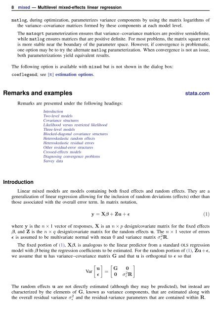
Linear mixed models are models containing both fixed effects and random effects. They are a
generalization of linear regression allowing for the inclusion of random deviations (effects) other than
those associated with the overall error term. In matrix notation,
y = Xβ + Zu + ɛ (1)
where y is the n × 1 vector of responses, X is an n × p design/covariate matrix for the fixed effects
β, and Z is the n × q design/covariate matrix for the random effects u. The n × 1 vector of errors
ɛ is assumed to be multivariate normal with mean 0 and variance matrix σ 2 ɛ R.
The fixed portion of (1), Xβ, is analogous to the linear predictor from a standard OLS regression
model with β being the regression coefficients to be estimated. For the random portion of (1), Zu+ɛ,
we assume that u has variance–covariance matrix G and that u is orthogonal to ɛ so that
[ ]
u
Var =
ɛ
[
G 0
]
0 σɛ 2 R
The random effects u are not directly estimated (although they may be predicted), but instead are
characterized by the elements of G, known as variance components, that are estimated along with
the overall residual variance σɛ 2 and the residual-variance parameters that are contained within R.