

mixed - Stata
mixed - Stata
mixed - Stata

Create successful ePaper yourself
Turn your PDF publications into a flip-book with our unique Google optimized e-Paper software.
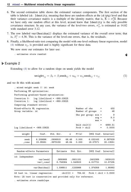
12 <strong>mixed</strong> — Multilevel <strong>mixed</strong>-effects linear regression<br />
6. The second estimation table shows the estimated variance components. The first section of the<br />
table is labeled id: Identity, meaning that these are random effects at the id (pig) level and that<br />
their variance–covariance matrix is a multiple of the identity matrix; that is, Σ = σuI. 2 Because<br />
we have only one random effect at this level, <strong>mixed</strong> knew that Identity is the only possible<br />
covariance structure. In any case, the variance of the level-two errors, σu 2 , is estimated as 14.82<br />
with standard error 3.12.<br />
7. The row labeled var(Residual) displays the estimated variance of the overall error term; that<br />
is, ̂σ 2 ɛ = 4.38. This is the variance of the level-one errors, that is, the residuals.<br />
8. Finally, a likelihood-ratio test comparing the model with one-level ordinary linear regression, model<br />
(4) without u j , is provided and is highly significant for these data.<br />
We now store our estimates for later use:<br />
. estimates store randint<br />
Example 2<br />
Extending (4) to allow for a random slope on week yields the model<br />
and we fit this with <strong>mixed</strong>:<br />
. <strong>mixed</strong> weight week || id: week<br />
Performing EM optimization:<br />
weight ij = β 0 + β 1 week ij + u 0j + u 1j week ij + ɛ ij (5)<br />
Performing gradient-based optimization:<br />
Iteration 0: log likelihood = -869.03825<br />
Iteration 1: log likelihood = -869.03825<br />
Computing standard errors:<br />
Mixed-effects ML regression Number of obs = 432<br />
Group variable: id Number of groups = 48<br />
Obs per group: min = 9<br />
avg = 9.0<br />
max = 9<br />
Wald chi2(1) = 4689.51<br />
Log likelihood = -869.03825 Prob > chi2 = 0.0000<br />
weight Coef. Std. Err. z P>|z| [95% Conf. Interval]<br />
week 6.209896 .0906819 68.48 0.000 6.032163 6.387629<br />
_cons 19.35561 .3979159 48.64 0.000 18.57571 20.13551<br />
Random-effects Parameters Estimate Std. Err. [95% Conf. Interval]<br />
id: Independent<br />
var(week) .3680668 .0801181 .2402389 .5639103<br />
var(_cons) 6.756364 1.543503 4.317721 10.57235<br />
var(Residual) 1.598811 .1233988 1.374358 1.85992<br />
LR test vs. linear regression: chi2(2) = 764.42 Prob > chi2 = 0.0000<br />
Note: LR test is conservative and provided only for reference.<br />
. estimates store randslope


