mixed - Stata

More documents

Recommendations

Info

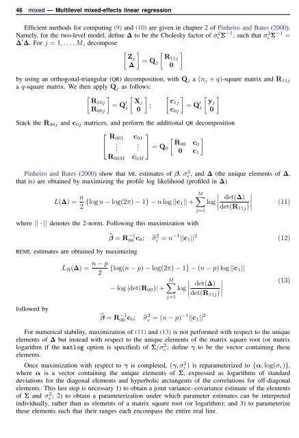
46 mixed — Multilevel mixed-effects linear regression Efficient methods for computing (9) and (10) are given in chapter 2 of Pinheiro and Bates (2000). Namely, for the two-level model, define ∆ to be the Cholesky factor of σɛ 2Σ−1 , such that σɛ 2Σ−1 = ∆ ′ ∆. For j = 1, . . . , M, decompose [ ] [ ] Zj R11j = Q ∆ j 0 by using an orthogonal-triangular (QR) decomposition, with Q j a (n j + q)-square matrix and R 11j a q-square matrix. We then apply Q j as follows: [ ] [ ] [ ] [ ] R10j = Q ′ Xj c1j j ; = Q ′ yj j R 00j 0 c 0j 0 Stack the R 00j and c 0j matrices, and perform the additional QR decomposition ⎡ ⎤ R 001 c 01 [ ] ⎣ . ⎦ R00 c . = Q 0 0 0 c 1 c 0M R 00M Pinheiro and Bates (2000) show that ML estimates of β, σɛ 2 , and ∆ (the unique elements of ∆, that is) are obtained by maximizing the profile log likelihood (profiled in ∆) L(∆) = n 2 {log n − log(2π) − 1} − n log ||c 1|| + where || · || denotes the 2-norm. Following this maximization with REML estimates are obtained by maximizing followed by L R (∆) = n − p 2 M∑ log det(∆) ∣det(R 11j ) ∣ (11) j=1 ̂β = R −1 00 c 0; ̂σ 2 ɛ = n −1 ||c 1 || 2 (12) {log(n − p) − log(2π) − 1} − (n − p) log ||c 1 || − log |det(R 00 )| + M∑ log det(∆) ∣det(R 11j ) ∣ j=1 ̂β = R −1 00 c 0; ̂σ 2 ɛ = (n − p) −1 ||c 1 || 2 For numerical stability, maximization of (11) and (13) is not performed with respect to the unique elements of ∆ but instead with respect to the unique elements of the matrix square root (or matrix logarithm if the matlog option is specified) of Σ/σɛ 2 ; define γ to be the vector containing these elements. Once maximization with respect to γ is completed, (γ, σɛ 2 ) is reparameterized to {α, log(σ ɛ )}, where α is a vector containing the unique elements of Σ, expressed as logarithms of standard deviations for the diagonal elements and hyperbolic arctangents of the correlations for off-diagonal elements. This last step is necessary 1) to obtain a joint variance–covariance estimate of the elements of Σ and σɛ 2 ; 2) to obtain a parameterization under which parameter estimates can be interpreted individually, rather than as elements of a matrix square root (or logarithm); and 3) to parameterize these elements such that their ranges each encompass the entire real line. (13)
mixed — Multilevel mixed-effects linear regression 47 Obtaining a joint variance–covariance matrix for the estimated {α, log(σ ɛ )} requires the evaluation of the log likelihood (or log-restricted likelihood) with only β profiled out. For ML, we have L ∗ {α, log(σ ɛ )} = L{∆(α, σɛ 2 ), σɛ 2 } = − n 2 log(2πσ2 ɛ ) − ||c 1|| 2 M∑ + log det(∆) ∣det(R 11j ) ∣ with the analogous expression for REML. The variance–covariance matrix of ̂β is estimated as ̂Var(̂β) = ̂σ 2 ɛ R −1 00 2σ 2 ɛ ( ) R −1 ′ 00 but this does not mean that ̂Var(̂β) is identical under both ML and REML because R00 depends on ∆. Because ̂β is asymptotically uncorrelated with {̂α, log(̂σɛ )}, the covariance of ̂β with the other estimated parameters is treated as 0. Parameter estimates are stored in e(b) as {̂β, ̂α, log(̂σɛ )}, with the corresponding (block-diagonal) variance–covariance matrix stored in e(V). Parameter estimates can be displayed in this metric by specifying the estmetric option. However, in mixed output, variance components are most often displayed either as variances and covariances or as standard deviations and correlations. EM iterations are derived by considering the u j in (2) as missing data. Here we describe the procedure for maximizing the log likelihood via EM; the procedure for maximizing the restricted log likelihood is similar. The log likelihood for the full data (y, u) is L F (β, Σ, σ 2 ɛ ) = j=1 M∑ { log f1 (y j |u j , β, σɛ 2 ) + log f 2 (u j |Σ) } j=1 where f 1 (·) is the density function for multivariate normal with mean X j β + Z j u j and variance σɛ 2 I nj , and f 2 (·) is the density for multivariate normal with mean 0 and q × q covariance matrix Σ. As before, we can profile β and σɛ 2 out of the optimization, yielding the following EM iterative procedure: 1. For the current iterated value of Σ (t) , fix ̂β = ̂β(Σ (t) ) and ̂σ 2 ɛ = ̂σ 2 ɛ (Σ (t) ) according to (12). 2. Expectation step: Calculate { } D(Σ) ≡ E L F (̂β, Σ, ̂σ 2 ɛ )|y = C − M 2 log det (Σ) − 1 2 M∑ E ( u ′ j Σ−1 u j |y ) where C is a constant that does not depend on Σ, and the expected value of the quadratic form u ′ j Σ−1 u j is taken with respect to the conditional density f(u j |y, ̂β, Σ (t) , ̂σ 2 ɛ ). 3. Maximization step: Maximize D(Σ) to produce Σ (t+1) . j=1
Page 1 and 2: Title stata.com mixed — Multileve
Page 3 and 4: vartype Description mixed — Multi
Page 5 and 6: mixed — Multilevel mixed-effects
Page 45: mixed — Multilevel mixed-effects
Page 51: Also see mixed — Multilevel mixed

mixed - Stata

You also want an ePaper? Increase the reach of your titles

Delete template?

Save as template?