meoprobit - Stata

Title
stata.com
meoprobit — Multilevel mixed-effects ordered probit regression
Syntax Menu Description Options
Remarks and examples Stored results Methods and formulas References
Also see
Syntax
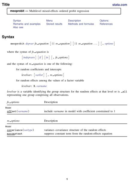
meoprobit depvar fe equation [ || re equation ] [ || re equation . . . ] [ , options ]
where the syntax of fe equation is
[
indepvars
] [
if
] [
in
] [
, fe options
]
and the syntax of re equation is one of the following:
for random coefficients and intercepts
levelvar: [ varlist ] [ , re options ]
for random effects among the values of a factor variable
levelvar: R.varname
levelvar is a variable identifying the group structure for the random effects at that level or is
representing one group comprising all observations.
all
fe options
Description
Model
offset(varname) include varname in model with coefficient constrained to 1
re options
Model
covariance(vartype)
noconstant
Description
variance–covariance structure of the random effects
suppress constant term from the random-effects equation
1

2 meoprobit — Multilevel mixed-effects ordered probit regression
options
Model
constraints(constraints)
collinear
SE/Robust
vce(vcetype)
Reporting
level(#)
nocnsreport
notable
noheader
nogroup
nolrtest
display options
Integration
intmethod(intmethod)
intpoints(#)
Maximization
maximize options
startvalues(svmethod)
startgrid [ (gridspec) ]
noestimate
dnumerical
coeflegend
Description
apply specified linear constraints
keep collinear variables
vcetype may be oim, robust, or cluster clustvar
set confidence level; default is level(95)
do not display constraints
suppress coefficient table
suppress output header
suppress table summarizing groups
do not perform likelihood-ratio test comparing with ordered probit
regression
control column formats, row spacing, line width, display of omitted
variables and base and empty cells, and factor-variable labeling
integration method
set the number of integration (quadrature) points for all levels;
default is intpoints(7)
control the maximization process; seldom used
method for obtaining starting values
perform a grid search to improve starting values
do not fit the model; show starting values instead
use numerical derivative techniques
display legend instead of statistics
vartype
independent
exchangeable
identity
unstructured
fixed(matname)
pattern(matname)
Description
one unique variance parameter per random effect, all covariances
0; the default unless the R. notation is used
equal variances for random effects, and one common pairwise
covariance
equal variances for random effects, all covariances 0; the
default if the R. notation is used
all variances and covariances to be distinctly estimated
user-selected variances and covariances constrained to specified
values; the remaining variances and covariances unrestricted
user-selected variances and covariances constrained to be equal;
the remaining variances and covariances unrestricted

meoprobit — Multilevel mixed-effects ordered probit regression 3
intmethod
mvaghermite
mcaghermite
ghermite
laplace
Description
mean-variance adaptive Gauss–Hermite quadrature; the default
unless a crossed random-effects model is fit
mode-curvature adaptive Gauss–Hermite quadrature
nonadaptive Gauss–Hermite quadrature
Laplacian approximation; the default for crossed random-effects
models
indepvars may contain factor variables; see [U] 11.4.3 Factor variables.
depvar, indepvars, and varlist may contain time-series operators; see [U] 11.4.4 Time-series varlists.
by is allowed; see [U] 11.1.10 Prefix commands.
startvalues(), startgrid, noestimate, dnumerical, and coeflegend do not appear in the dialog box.
See [U] 20 Estimation and postestimation commands for more capabilities of estimation commands.
Menu
Statistics > Multilevel mixed-effects models > Ordered probit regression
Description
meoprobit fits mixed-effects probit models for ordered responses. The actual values taken on by
the response are irrelevant except that larger values are assumed to correspond to “higher” outcomes.
The conditional distribution of the response given the random effects is assumed to be multinomial,
with success probability determined by the standard normal cumulative distribution function.
Options
✄
✄
Model
offset(varname) specifies that varname be included in the fixed-effects portion of the model with
the coefficient constrained to be 1.
covariance(vartype) specifies the structure of the covariance matrix for the random effects and
may be specified for each random-effects equation. vartype is one of the following: independent,
exchangeable, identity, unstructured, fixed(matname), or pattern(matname).
covariance(independent) covariance structure allows for a distinct variance for each random
effect within a random-effects equation and assumes that all covariances are 0. The default is
covariance(independent) unless a crossed random-effects model is fit, in which case the
default is covariance(identity).
covariance(exchangeable) structure specifies one common variance for all random effects and
one common pairwise covariance.
covariance(identity) is short for “multiple of the identity”; that is, all variances are equal
and all covariances are 0.
covariance(unstructured) allows for all variances and covariances to be distinct. If an equation
consists of p random-effects terms, the unstructured covariance matrix will have p(p + 1)/2
unique parameters.

4 meoprobit — Multilevel mixed-effects ordered probit regression
✄
covariance(fixed(matname)) and covariance(pattern(matname)) covariance structures
provide a convenient way to impose constraints on variances and covariances of random effects.
Each specification requires a matname that defines the restrictions placed on variances and
covariances. Only elements in the lower triangle of matname are used, and row and column names
of matname are ignored. A missing value in matname means that a given element is unrestricted.
In a fixed(matname) covariance structure, (co)variance (i, j) is constrained to equal the
value specified in the i, jth entry of matname. In a pattern(matname) covariance structure,
(co)variances (i, j) and (k, l) are constrained to be equal if matname[i, j] = matname[k, l].
noconstant suppresses the constant (intercept) term; may be specified for any or all of the randomeffects
equations.
constraints(constraints), collinear; see [R] estimation options.
✄
SE/Robust
vce(vcetype) specifies the type of standard error reported, which includes types that are derived
from asymptotic theory (oim), that are robust to some kinds of misspecification (robust), and
that allow for intragroup correlation (cluster clustvar); see [R] vce option. If vce(robust) is
specified, robust variances are clustered at the highest level in the multilevel model.
✄
✄ Reporting
level(#), nocnsreport; see [R] estimation options.
✄
notable suppresses the estimation table, either at estimation or upon replay.
noheader suppresses the output header, either at estimation or upon replay.
nogroup suppresses the display of group summary information (number of groups, average group
size, minimum, and maximum) from the output header.
nolrtest prevents meoprobit from performing a likelihood-ratio test that compares the mixed-effects
ordered probit model with standard (marginal) ordered probit regression. This option may also be
specified upon replay to suppress this test from the output.
display options: noomitted, vsquish, noemptycells, baselevels, allbaselevels, nofvlabel,
fvwrap(#), fvwrapon(style), cformat(% fmt), pformat(% fmt), sformat(% fmt), and
nolstretch; see [R] estimation options.
✄
Integration
intmethod(intmethod) specifies the integration method to be used for the random-effects model.
mvaghermite performs mean and variance adaptive Gauss–Hermite quadrature; mcaghermite
performs mode and curvature adaptive Gauss–Hermite quadrature; ghermite performs nonadaptive
Gauss–Hermite quadrature; and laplace performs the Laplacian approximation, equivalent to mode
curvature adaptive Gaussian quadrature with one integration point.
The default integration method is mvaghermite unless a crossed random-effects model is fit, in
which case the default integration method is laplace. The Laplacian approximation has been
known to produce biased parameter estimates; however, the bias tends to be more prominent in
the estimates of the variance components rather than in the estimates of the fixed effects.
For crossed random-effects models, estimation with more than one quadrature point may be
prohibitively intensive even for a small number of levels. For this reason, the integration method
defaults to the Laplacian approximation. You may override this behavior by specifying a different
integration method.

meoprobit — Multilevel mixed-effects ordered probit regression 5
✄
intpoints(#) sets the number of integration points for quadrature. The default is intpoints(7),
which means that seven quadrature points are used for each level of random effects. This option
is not allowed with intmethod(laplace).
The more integration points, the more accurate the approximation to the log likelihood. However,
computation time increases as a function of the number of quadrature points raised to a power
equaling the dimension of the random-effects specification. In crossed random-effects models and
in models with many levels or many random coefficients, this increase can be substantial.
✄
Maximization
maximize options: difficult, technique(algorithm spec), iterate(#), [ no ] log, trace,
gradient, showstep, hessian, showtolerance, tolerance(#), ltolerance(#),
nrtolerance(#), nonrtolerance, and from(init specs); see [R] maximize. Those that require
special mention for meoprobit are listed below.
from() accepts a properly labeled vector of initial values or a list of coefficient names with values.
A list of values is not allowed.
The following options are available with meoprobit but are not shown in the dialog box:
startvalues(svmethod), startgrid [ (gridspec) ] , noestimate, and dnumerical; see [ME]
meglm.
coeflegend; see [R] estimation options.
Remarks and examples
For a general introduction to me commands, see [ME] me.
stata.com
meoprobit is a convenience command for meglm with a probit link and an ordinal family;
see [ME] meglm.
Remarks are presented under the following headings:
Introduction
Two-level models
Three-level models
Introduction
Mixed-effects ordered probit regression is ordered probit regression containing both fixed effects
and random effects. An ordered response is a variable that is categorical and ordered, for instance,
“poor”, “good”, and “excellent”, which might indicate a person’s current health status or the repair
record of a car. In the absence of random effects, mixed-effects ordered probit regression reduces to
ordered probit regression; see [R] oprobit.
Comprehensive treatments of mixed models are provided by, for example, Searle, Casella, and Mc-
Culloch (1992); Verbeke and Molenberghs (2000); Raudenbush and Bryk (2002); Demidenko (2004);
Hedeker and Gibbons (2006); McCulloch, Searle, and Neuhaus (2008); and Rabe-Hesketh and Skrondal
(2012). Agresti (2010, chap. 10) and Rabe-Hesketh and Skrondal (2012, chap. 11) are good
introductory readings on applied multilevel modeling of ordinal data.
meoprobit allows for many levels of nested clusters of random effects. For example, in a threelevel
model you can specify random effects for schools and then random effects for classes nested
within schools. In this model, the observations (presumably, the students) comprise the first level, the
classes comprise the second level, and the schools comprise the third.

6 meoprobit — Multilevel mixed-effects ordered probit regression
However, for simplicity, for now we consider the two-level model, where for a series of M
independent clusters, and conditional on a set of fixed effects x ij , a set of cutpoints κ, and a set of
random effects u j , the cumulative probability of the response being in a category higher than k is
Pr(y ij > k|x ij , κ, u j ) = Φ(x ij β + z ij u j − κ k ) (1)
for j = 1, . . . , M clusters, with cluster j consisting of i = 1, . . . , n j observations. The cutpoints
are labeled κ 1 , κ 2 , . . . , κ K−1 , where K is the number of possible outcomes. Φ(·) is the standard
normal cumulative distribution function that represents cumulative probability.
The 1 × p row vector x ij are the covariates for the fixed effects, analogous to the covariates you
would find in a standard probit regression model, with regression coefficients (fixed effects) β. In our
parameterization, x ij does not contain a constant term because its effect is absorbed into the cutpoints.
For notational convenience here and throughout this manual entry, we suppress the dependence of
y ij on x ij .
The 1 × q vector z ij are the covariates corresponding to the random effects and can be used to
represent both random intercepts and random coefficients. For example, in a random-intercept model,
z ij is simply the scalar 1. The random effects u j are M realizations from a multivariate normal
distribution with mean 0 and q × q variance matrix Σ. The random effects are not directly estimated
as model parameters but are instead summarized according to the unique elements of Σ, known
as variance components. One special case of (1) places z ij = x ij so that all covariate effects are
essentially random and distributed as multivariate normal with mean β and variance Σ.
From (1), we can derive the probability of observing outcome k as
Pr(y ij = k|κ, u j ) = Pr(κ k−1 < x ij β + z ij u j + ɛ ij ≤ κ k )
where κ 0 is taken as −∞ and κ K is taken as +∞.
= Pr(κ k−1 − x ij β − z ij u j < ɛ ij ≤ κ k − x ij β − z ij u j )
= Φ(κ k − x ij β − z ij u j ) − Φ(κ k−1 − x ij β − z ij u j )
From the above, we may also write the model in terms of a latent linear response, where observed
ordinal responses y ij are generated from the latent continuous responses, such that
y ∗ ij = x ij β + z ij u j + ɛ ij
and
⎧
1 if yij ∗
⎪⎨
≤ κ 1
2 if κ 1 < yij ∗ ≤ κ 2
y ij =
. ⎪⎩
K if κ K−1 < yij
∗
The errors ɛ ij are distributed as standard normal with mean 0 and variance 1 and are independent of
u j .
Model (1) is an example of a generalized linear mixed model (GLMM), which generalizes the
linear mixed-effects (LME) model to non-Gaussian responses. You can fit LMEs in Stata by using
mixed and fit GLMMs by using meglm. Because of the relationship between LMEs and GLMMs, there
is insight to be gained through examination of the linear mixed model. This is especially true for
Stata users because the terminology, syntax, options, and output for fitting these types of models are
nearly identical. See [ME] mixed and the references therein, particularly in the Introduction, for more
information.

meoprobit — Multilevel mixed-effects ordered probit regression 7
Log-likelihood calculations for fitting any generalized mixed-effects model require integrating out
the random effects. One widely used modern method is to directly estimate the integral required to
calculate the log likelihood by Gauss–Hermite quadrature or some variation thereof. Because the log
likelihood itself is estimated, this method has the advantage of permitting likelihood-ratio tests for
comparing nested models. Also, if done correctly, quadrature approximations can be quite accurate,
thus minimizing bias.
meoprobit supports three types of Gauss–Hermite quadrature and the Laplacian approximation
method; see Methods and formulas of [ME] meglm for details.
Below we present two short examples of mixed-effects ordered probit regression; refer to [ME] melogit
for additional examples including crossed random-effects models and to [ME] me and [ME] meglm
for examples of other random-effects models.
Two-level models
We begin with a simple application of (1) as a two-level model, because a one-level model, in our
terminology, is just standard ordered probit regression; see [R] oprobit.
Example 1
We use the data from the Television, School, and Family Smoking Prevention and Cessation Project
(Flay et al. 1988; Rabe-Hesketh and Skrondal 2012, chap. 11), where schools were randomly assigned
into one of four groups defined by two treatment variables. Students within each school are nested in
classes, and classes are nested in schools. In this example, we ignore the variability of classes within
schools and fit a two-level model; we incorporate classes in a three-level model in example 2. The
dependent variable is the tobacco and health knowledge (THK) scale score collapsed into four ordered
categories. We regress the outcome on the treatment variables and their interaction and control for
the pretreatment score.

8 meoprobit — Multilevel mixed-effects ordered probit regression
. use http://www.stata-press.com/data/r13/tvsfpors
. meoprobit thk prethk cc##tv || school:
Fitting fixed-effects model:
Iteration 0: log likelihood = -2212.775
Iteration 1: log likelihood = -2127.8111
Iteration 2: log likelihood = -2127.7612
Iteration 3: log likelihood = -2127.7612
Refining starting values:
Grid node 0: log likelihood = -2149.7302
Fitting full model:
Iteration 0: log likelihood = -2149.7302 (not concave)
Iteration 1: log likelihood = -2129.6838 (not concave)
Iteration 2: log likelihood = -2123.5143
Iteration 3: log likelihood = -2122.2896
Iteration 4: log likelihood = -2121.7949
Iteration 5: log likelihood = -2121.7716
Iteration 6: log likelihood = -2121.7715
Mixed-effects oprobit regression Number of obs = 1600
Group variable: school Number of groups = 28
Obs per group: min = 18
avg = 57.1
max = 137
Integration method: mvaghermite Integration points = 7
Wald chi2(4) = 128.05
Log likelihood = -2121.7715 Prob > chi2 = 0.0000
thk Coef. Std. Err. z P>|z| [95% Conf. Interval]
prethk .2369804 .0227739 10.41 0.000 .1923444 .2816164
1.cc .5490957 .1255108 4.37 0.000 .303099 .7950923
1.tv .1695405 .1215889 1.39 0.163 -.0687693 .4078504
cc#tv
1 1 -.2951837 .1751969 -1.68 0.092 -.6385634 .0481959
/cut1 -.0682011 .1003374 -0.68 0.497 -.2648587 .1284565
/cut2 .67681 .1008836 6.71 0.000 .4790817 .8745382
/cut3 1.390649 .1037494 13.40 0.000 1.187304 1.593995
school
var(_cons) .0288527 .0146201 .0106874 .0778937
LR test vs. oprobit regression: chibar2(01) = 11.98 Prob>=chibar2 = 0.0003
Those of you familiar with the mixed command or other me commands will recognize the syntax
and output. Below we comment on the items specific to ordered outcomes.
1. The estimation table reports the fixed effects, the estimated cutpoints (κ 1 , κ 2 , κ 3 ), and the
estimated variance components. The fixed effects can be interpreted just as you would the output
from oprobit. We find that students with higher preintervention scores tend to have higher
postintervention scores. Because of their interaction, the impact of the treatment variables on the
knowledge score is not straightforward; we defer this discussion to example 1 of [ME] meoprobit
postestimation.
2. Underneath the fixed effects and the cutpoints, the table shows the estimated variance components.
The random-effects equation is labeled school, meaning that these are random effects at the school
level. Because we have only one random effect at this level, the table shows only one variance

meoprobit — Multilevel mixed-effects ordered probit regression 9
component. The estimate of σu 2 is 0.03 with standard error 0.01. The reported likelihood-ratio test
shows that there is enough variability between schools to favor a mixed-effects ordered probit
regression over a standard ordered probit regression; see Distribution theory for likelihood-ratio
test in [ME] me for a discussion of likelihood-ratio testing of variance components.
We now store our estimates for later use.
. estimates store r_2
Three-level models
Two-level models extend naturally to models with three or more levels with nested random effects.
Below we continue with example 1.
Example 2
In this example, we fit a three-level model incorporating classes nested within schools as an
additional level. The fixed-effects part remains the same.

10 meoprobit — Multilevel mixed-effects ordered probit regression
Notes:
. meoprobit thk prethk cc##tv || school: || class:
Fitting fixed-effects model:
Iteration 0: log likelihood = -2212.775
Iteration 1: log likelihood = -2127.8111
Iteration 2: log likelihood = -2127.7612
Iteration 3: log likelihood = -2127.7612
Refining starting values:
Grid node 0: log likelihood = -2195.6424
Fitting full model:
Iteration 0: log likelihood = -2195.6424 (not concave)
Iteration 1: log likelihood = -2167.9576 (not concave)
Iteration 2: log likelihood = -2140.2644 (not concave)
Iteration 3: log likelihood = -2128.6948 (not concave)
Iteration 4: log likelihood = -2119.9225
Iteration 5: log likelihood = -2117.0947
Iteration 6: log likelihood = -2116.7004
Iteration 7: log likelihood = -2116.6981
Iteration 8: log likelihood = -2116.6981
Mixed-effects oprobit regression Number of obs = 1600
No. of Observations per Group
Group Variable Groups Minimum Average Maximum
school 28 18 57.1 137
class 135 1 11.9 28
Integration method: mvaghermite Integration points = 7
Wald chi2(4) = 124.20
Log likelihood = -2116.6981 Prob > chi2 = 0.0000
thk Coef. Std. Err. z P>|z| [95% Conf. Interval]
prethk .238841 .0231446 10.32 0.000 .1934784 .2842036
1.cc .5254813 .1285816 4.09 0.000 .2734659 .7774967
1.tv .1455573 .1255827 1.16 0.246 -.1005803 .3916949
cc#tv
1 1 -.2426203 .1811999 -1.34 0.181 -.5977656 .1125251
/cut1 -.074617 .1029791 -0.72 0.469 -.2764523 .1272184
/cut2 .6863046 .1034813 6.63 0.000 .4834849 .8891242
/cut3 1.413686 .1064889 13.28 0.000 1.204972 1.622401
school
var(_cons) .0186456 .0160226 .0034604 .1004695
school>class
var(_cons) .0519974 .0224014 .0223496 .1209745
LR test vs. oprobit regression: chi2(2) = 22.13 Prob > chi2 = 0.0000
Note: LR test is conservative and provided only for reference.
1. Our model now has two random-effects equations, separated by ||. The first is a random intercept
(constant only) at the school level (level three), and the second is a random intercept at the
class level (level two). The order in which these are specified (from left to right) is significant—
meoprobit assumes that class is nested within school.

meoprobit — Multilevel mixed-effects ordered probit regression 11
2. The information on groups is now displayed as a table, with one row for each grouping. You can
suppress this table with the nogroup or the noheader option, which will suppress the rest of the
header as well.
3. The variance-component estimates are now organized and labeled according to level. The variance
component for class is labeled school>class to emphasize that classes are nested within schools.
Compared with the two-level model from example 1, the estimate of the random intercept at the
school level dropped from 0.03 to 0.02. This is not surprising because we now use two random
components versus one random component to account for unobserved heterogeneity among students.
We can use lrtest and our stored estimation result from example 1 to see which model provides a
better fit:
. lrtest r_2 .
Likelihood-ratio test LR chi2(1) = 10.15
(Assumption: r_2 nested in .) Prob > chi2 = 0.0014
Note: The reported degrees of freedom assumes the null hypothesis is not on
the boundary of the parameter space. If this is not true, then the
reported test is conservative.
The likelihood-ratio test favors the three-level model. For more information about the likelihoodratio
test in the context of mixed-effects models, see Distribution theory for likelihood-ratio test in
[ME] me.
The above extends to models with more than two levels of nesting in the obvious manner, by
adding more random-effects equations, each separated by ||. The order of nesting goes from left to
right as the groups go from biggest (highest level) to smallest (lowest level).
Stored results
meoprobit stores the following in e():
Scalars
e(N)
number of observations
e(k)
number of parameters
e(k dv)
number of dependent variables
e(k cat)
number of categories
e(k eq)
number of equations in e(b)
e(k eq model)
number of equations in overall model test
e(k f)
number of fixed-effects parameters
e(k r)
number of random-effects parameters
e(k rs)
number of variances
e(k rc)
number of covariances
e(df m)
model degrees of freedom
e(ll)
log likelihood
e(N clust)
number of clusters
e(chi2) χ 2
e(p)
significance
e(ll c)
log likelihood, comparison model
e(chi2 c)
χ 2 , comparison model
e(df c)
degrees of freedom, comparison model
e(p c)
significance, comparison model
e(rank)
rank of e(V)
e(ic)
number of iterations
e(rc)
return code
e(converged)
1 if converged, 0 otherwise

12 meoprobit — Multilevel mixed-effects ordered probit regression
Macros
e(cmd)
meoprobit
e(cmdline)
command as typed
e(depvar)
name of dependent variable
e(covariates)
list of covariates
e(ivars)
grouping variables
e(model)
oprobit
e(title)
title in estimation output
e(link)
probit
e(family)
ordinal
e(clustvar)
name of cluster variable
e(offset)
offset
e(intmethod)
integration method
e(n quad)
number of integration points
e(chi2type) Wald; type of model χ 2
e(vce)
vcetype specified in vce()
e(vcetype)
title used to label Std. Err.
e(opt)
type of optimization
e(which)
max or min; whether optimizer is to perform maximization or minimization
e(ml method)
type of ml method
e(user)
name of likelihood-evaluator program
e(technique)
maximization technique
e(datasignature) the checksum
e(datasignaturevars) variables used in calculation of checksum
e(properties)
b V
e(estat cmd)
program used to implement estat
e(predict)
program used to implement predict
Matrices
e(b)
e(Cns)
e(ilog)
e(gradient)
e(N g)
e(g min)
e(g avg)
e(g max)
e(V)
e(V modelbased)
Functions
e(sample)
coefficient vector
constraints matrix
iteration log (up to 20 iterations)
gradient vector
group counts
group-size minimums
group-size averages
group-size maximums
variance–covariance matrix of the estimator
model-based variance
marks estimation sample
Methods and formulas
Without a loss of generality, consider a two-level ordered probit model. The probability of observing
outcome k for response y ij is then
p ij = Pr(y ij = k|κ, u j ) = Pr(κ k−1 < η ij + ɛ it ≤ κ k )
= Φ(κ k − η ij ) − Φ(κ k−1 − η ij )
where η ij = x ij β + z ij u j + offset ij , κ 0 is taken as −∞, and κ K is taken as +∞. Here x ij does
not contain a constant term because its effect is absorbed into the cutpoints.
For cluster j, j = 1, . . . , M, the conditional distribution of y j = (y j1 , . . . , y jnj ) ′ given a set of
cluster-level random effects u j is

meoprobit — Multilevel mixed-effects ordered probit regression 13
n j
∏
f(y j |u j ) =
i=1
p I k(y ij)
ij
n
∑ j {
}
= exp I k (y ij ) log(p ij )
i=1
where
I k (y ij ) =
{ 1 if yij = k
0 otherwise
Because the prior distribution of u j is multivariate normal with mean 0 and q × q variance matrix
Σ, the likelihood contribution for the jth cluster is obtained by integrating u j out of the joint density
f(y j , u j ),
L j (β, κ, Σ) = (2π) −q/2 |Σ| −1/2 ∫
= (2π) −q/2 |Σ| −1/2 ∫
f(y j |κ, u j ) exp ( −u ′ j Σ−1 u j /2 ) du j
exp {g (β, κ, Σ, u j )} du j
(2)
where
n
∑ j {
}
g (β, κ, Σ, u j ) = I k (y ij ) log(p ij ) − u ′ j Σ−1 u j /2
i=1
and for convenience, in the arguments of g(·) we suppress the dependence on the observable data
(y j , r j , X j , Z j ).
The integration in (2) has no closed form and thus must be approximated. meoprobit offers
four approximation methods: mean–variance adaptive Gauss–Hermite quadrature (default unless a
crossed random-effects model is fit), mode-curvature adaptive Gauss–Hermite quadrature, nonadaptive
Gauss–Hermite quadrature, and Laplacian approximation (default for crossed random-effects models).
The Laplacian approximation is based on a second-order Taylor expansion of g (β, κ, Σ, u j ) about
the value of u j that maximizes it; see Methods and formulas in [ME] meglm for details.
Gaussian quadrature relies on transforming the multivariate integral in (2) into a set of nested
univariate integrals. Each univariate integral can then be evaluated using a form of Gaussian quadrature;
see Methods and formulas in [ME] meglm for details.
The log likelihood for the entire dataset is simply the sum of the contributions of the M individual
clusters, namely, L(β, κ, Σ) = ∑ M
j=1 L j(β, κ, Σ).
Maximization of L(β, κ, Σ) is performed with respect to (β, κ, σ 2 ), where σ 2 is a vector comprising
the unique elements of Σ. Parameter estimates are stored in e(b) as (̂β, ̂κ, ̂σ 2 ), with the corresponding
variance–covariance matrix stored in e(V).
References
Agresti, A. 2010. Analysis of Ordinal Categorical Data. 2nd ed. Hoboken, NJ: Wiley.
Andrews, M. J., T. Schank, and R. Upward. 2006. Practical fixed-effects estimation methods for the three-way
error-components model. Stata Journal 6: 461–481.
Demidenko, E. 2004. Mixed Models: Theory and Applications. Hoboken, NJ: Wiley.

14 meoprobit — Multilevel mixed-effects ordered probit regression
Flay, B. R., B. R. Brannon, C. A. Johnson, W. B. Hansen, A. L. Ulene, D. A. Whitney-Saltiel, L. R. Gleason,
S. Sussman, M. D. Gavin, K. M. Glowacz, D. F. Sobol, and D. C. Spiegel. 1988. The television, school, and family
smoking cessation and prevention project: I. Theoretical basis and program development. Preventive Medicine 17:
585–607.
Gutierrez, R. G., S. L. Carter, and D. M. Drukker. 2001. sg160: On boundary-value likelihood-ratio tests. Stata
Technical Bulletin 60: 15–18. Reprinted in Stata Technical Bulletin Reprints, vol. 10, pp. 269–273. College Station,
TX: Stata Press.
Harbord, R. M., and P. Whiting. 2009. metandi: Meta-analysis of diagnostic accuracy using hierarchical logistic
regression. Stata Journal 9: 211–229.
Hedeker, D., and R. D. Gibbons. 2006. Longitudinal Data Analysis. Hoboken, NJ: Wiley.
Joe, H. 2008. Accuracy of Laplace approximation for discrete response mixed models. Computational Statistics &
Data Analysis 52: 5066–5074.
Laird, N. M., and J. H. Ware. 1982. Random-effects models for longitudinal data. Biometrics 38: 963–974.
Lin, X., and N. E. Breslow. 1996. Bias correction in generalized linear mixed models with multiple components of
dispersion. Journal of the American Statistical Association 91: 1007–1016.
Marchenko, Y. V. 2006. Estimating variance components in Stata. Stata Journal 6: 1–21.
McCulloch, C. E., S. R. Searle, and J. M. Neuhaus. 2008. Generalized, Linear, and Mixed Models. 2nd ed. Hoboken,
NJ: Wiley.
McLachlan, G. J., and K. E. Basford. 1988. Mixture Models. New York: Dekker.
Rabe-Hesketh, S., and A. Skrondal. 2012. Multilevel and Longitudinal Modeling Using Stata. 3rd ed. College Station,
TX: Stata Press.
Raudenbush, S. W., and A. S. Bryk. 2002. Hierarchical Linear Models: Applications and Data Analysis Methods.
2nd ed. Thousand Oaks, CA: Sage.
Searle, S. R., G. Casella, and C. E. McCulloch. 1992. Variance Components. New York: Wiley.
Self, S. G., and K.-Y. Liang. 1987. Asymptotic properties of maximum likelihood estimators and likelihood ratio tests
under nonstandard conditions. Journal of the American Statistical Association 82: 605–610.
Verbeke, G., and G. Molenberghs. 2000. Linear Mixed Models for Longitudinal Data. New York: Springer.
Also see
[ME] meoprobit postestimation — Postestimation tools for meoprobit
[ME] meologit — Multilevel mixed-effects ordered logistic regression
[ME] me — Introduction to multilevel mixed-effects models
[SEM] intro 5 — Tour of models (Multilevel mixed-effects models)
[XT] xtoprobit — Random-effects ordered probit models
[U] 20 Estimation and postestimation commands