meglm postestimation - Stata
meglm postestimation - Stata
meglm postestimation - Stata
You also want an ePaper? Increase the reach of your titles
YUMPU automatically turns print PDFs into web optimized ePapers that Google loves.
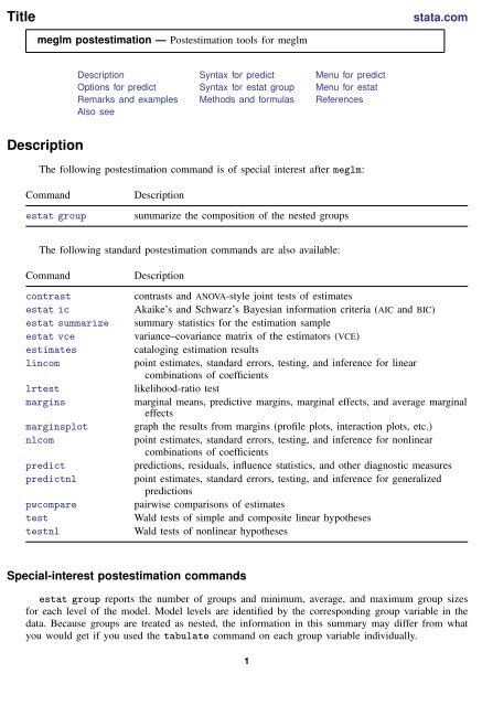
Title<br />
stata.com<br />
<strong>meglm</strong> <strong>postestimation</strong> — Postestimation tools for <strong>meglm</strong><br />
Description Syntax for predict Menu for predict<br />
Options for predict Syntax for estat group Menu for estat<br />
Remarks and examples Methods and formulas References<br />
Also see<br />
Description<br />
The following <strong>postestimation</strong> command is of special interest after <strong>meglm</strong>:<br />
Command<br />
estat group<br />
Description<br />
summarize the composition of the nested groups<br />
The following standard <strong>postestimation</strong> commands are also available:<br />
Command<br />
contrast<br />
estat ic<br />
estat summarize<br />
estat vce<br />
estimates<br />
lincom<br />
lrtest<br />
margins<br />
marginsplot<br />
nlcom<br />
predict<br />
predictnl<br />
pwcompare<br />
test<br />
testnl<br />
Description<br />
contrasts and ANOVA-style joint tests of estimates<br />
Akaike’s and Schwarz’s Bayesian information criteria (AIC and BIC)<br />
summary statistics for the estimation sample<br />
variance–covariance matrix of the estimators (VCE)<br />
cataloging estimation results<br />
point estimates, standard errors, testing, and inference for linear<br />
combinations of coefficients<br />
likelihood-ratio test<br />
marginal means, predictive margins, marginal effects, and average marginal<br />
effects<br />
graph the results from margins (profile plots, interaction plots, etc.)<br />
point estimates, standard errors, testing, and inference for nonlinear<br />
combinations of coefficients<br />
predictions, residuals, influence statistics, and other diagnostic measures<br />
point estimates, standard errors, testing, and inference for generalized<br />
predictions<br />
pairwise comparisons of estimates<br />
Wald tests of simple and composite linear hypotheses<br />
Wald tests of nonlinear hypotheses<br />
Special-interest <strong>postestimation</strong> commands<br />
estat group reports the number of groups and minimum, average, and maximum group sizes<br />
for each level of the model. Model levels are identified by the corresponding group variable in the<br />
data. Because groups are treated as nested, the information in this summary may differ from what<br />
you would get if you used the tabulate command on each group variable individually.<br />
1
2 <strong>meglm</strong> <strong>postestimation</strong> — Postestimation tools for <strong>meglm</strong><br />
Syntax for predict<br />
Syntax for obtaining predictions of random effects and their standard errors<br />
predict [ type ] newvarsspec [ if ] [ in ] , { remeans | remodes } [ reses(newvarsspec) ]<br />
Syntax for obtaining other predictions<br />
predict [ type ] newvarsspec [ if ] [ in ] [ , statistic options ]<br />
newvarsspec is stub* or newvarlist.<br />
statistic<br />
Main<br />
mu<br />
pr<br />
fitted<br />
xb<br />
stdp<br />
residuals<br />
pearson<br />
deviance<br />
anscombe<br />
Description<br />
mean response; the default<br />
synonym for mu for ordinal and binary response models<br />
fitted linear predictor<br />
linear predictor for the fixed portion of the model only<br />
standard error of the fixed-portion linear prediction<br />
raw residuals; available only with the Gaussian family<br />
Pearson residuals<br />
deviance residuals<br />
Anscombe residuals<br />
These statistics are available both in and out of sample; type predict . . . if e(sample) . . . if wanted<br />
only for the estimation sample.
<strong>meglm</strong> <strong>postestimation</strong> — Postestimation tools for <strong>meglm</strong> 3<br />
options<br />
Main<br />
means<br />
modes<br />
nooffset<br />
fixedonly<br />
outcome(outcome)<br />
Integration<br />
intpoints(#)<br />
iterate(#)<br />
tolerance(#)<br />
Description<br />
compute statistic using empirical Bayes means; the default<br />
compute statistic using empirical Bayes modes<br />
ignore the offset or exposure variable in calculating predictions; relevant only<br />
if you specified offset() or exposure() when you fit the model<br />
prediction for the fixed portion of the model only<br />
outcome category for predicted probabilities for ordinal models<br />
use # quadrature points to compute empirical Bayes means<br />
set maximum number of iterations in computing statistics involving<br />
empirical Bayes estimators<br />
set convergence tolerance for computing statistics involving empirical<br />
Bayes estimators<br />
For ordinal outcomes, you specify one or k new variables in newvarlist with mu and pr, where k is the number of<br />
outcomes. If you do not specify outcome(), those options assume outcome(#1).<br />
Menu for predict<br />
Statistics > Postestimation > Predictions, residuals, etc.<br />
Options for predict<br />
✄<br />
✄<br />
Main<br />
<br />
remeans calculates posterior means of the random effects, also known as empirical Bayes means.<br />
You must specify q new variables, where q is the number of random-effects terms in the model.<br />
However, it is much easier to just specify stub* and let <strong>Stata</strong> name the variables stub1, stub2, . . . ,<br />
stubq for you.<br />
remodes calculates posterior modes of the random effects, also known as empirical Bayes modes.<br />
You must specify q new variables, where q is the number of random-effects terms in the model.<br />
However, it is much easier to just specify stub* and let <strong>Stata</strong> name the variables stub1, stub2, . . . ,<br />
stubq for you.<br />
reses(stub* | newvarlist) calculates standard errors of the empirical Bayes estimators and stores the<br />
result in newvarlist. This option requires the remeans or the remodes option. You must specify q<br />
new variables, where q is the number of random-effects terms in the model. However, it is much<br />
easier to just specify stub* and let <strong>Stata</strong> name the variables stub1, stub2, . . . , stubq for you.<br />
The remeans, remodes, and reses() options often generate multiple new variables at once.<br />
When this occurs, the random effects (and standard errors) contained in the generated variables<br />
correspond to the order in which the variance components are listed in the output of <strong>meglm</strong>. Still,<br />
examining the variable labels of the generated variables (by using the describe command, for<br />
instance) can be useful in deciphering which variables correspond to which terms in the model.<br />
mu, the default, calculates the predicted mean, that is, the inverse link function applied to the linear<br />
prediction. By default, this is based on a linear predictor that includes both the fixed effects and<br />
the random effects, and the predicted mean is conditional on the values of the random effects. Use<br />
the fixedonly option if you want predictions that include only the fixed portion of the model,<br />
that is, if you want random effects set to 0.
4 <strong>meglm</strong> <strong>postestimation</strong> — Postestimation tools for <strong>meglm</strong><br />
✄<br />
pr calculates predicted probabilities and is a synonym for mu. This option is available only for ordinal<br />
and binary response models.<br />
fitted calculates the fitted linear prediction. By default, the fitted predictor includes both the fixed<br />
effects and the random effects. Use the fixedonly option if you want predictions that include<br />
only the fixed portion of the model, that is, if you want random effects set to 0.<br />
xb calculates the linear prediction xβ based on the estimated fixed effects (coefficients) in the model.<br />
This is equivalent to fixing all random effects in the model to their theoretical (prior) mean value<br />
of 0.<br />
stdp calculates the standard error of the fixed-effects linear predictor xβ.<br />
residuals calculates raw residuals, that is, responses minus the fitted values. This option is available<br />
only for the Gaussian family.<br />
pearson calculates Pearson residuals. Pearson residuals that are large in absolute value may indicate<br />
a lack of fit. By default, residuals include both the fixed portion and the random portion of the<br />
model. The fixedonly option modifies the calculation to include the fixed portion only.<br />
deviance calculates deviance residuals. Deviance residuals are recommended by McCullagh and<br />
Nelder (1989) as having the best properties for examining the goodness of fit of a GLM. They<br />
are approximately normally distributed if the model is correctly specified. They may be plotted<br />
against the fitted values or against a covariate to inspect the model fit. By default, residuals include<br />
both the fixed portion and the random portion of the model. The fixedonly option modifies the<br />
calculation to include the fixed portion only.<br />
anscombe calculates Anscombe residuals, which are designed to closely follow a normal distribution.<br />
By default, residuals include both the fixed portion and the random portion of the model. The<br />
fixedonly option modifies the calculation to include the fixed portion only.<br />
means specifies that posterior means be used as the estimates of the random effects for any statistic<br />
involving random effects. means is the default.<br />
modes specifies that posterior modes be used as the estimates of the random effects for any statistic<br />
involving random effects.<br />
nooffset is relevant only if you specified offset(varname o ) or exposure(varname e ) with<br />
<strong>meglm</strong>. It modifies the calculations made by predict so that they ignore the offset or the<br />
exposure variable; the linear prediction is treated as Xβ + Zu rather than Xβ + Zu + offset, or<br />
Xβ + Zu + ln(exposure), whichever is relevant.<br />
fixedonly modifies predictions to include only the fixed portion of the model, equivalent to setting<br />
all random effects equal to 0.<br />
outcome(outcome) specifies the outcome for which the predicted probabilities are to be calculated.<br />
outcome() should contain either one value of the dependent variable or one of #1, #2, . . . , with<br />
#1 meaning the first category of the dependent variable, #2 meaning the second category, etc.<br />
✄<br />
Integration<br />
<br />
intpoints(#) specifies the number of quadrature points used to compute the empirical Bayes means;<br />
the default is the value from estimation.<br />
iterate(#) specifies the maximum number of iterations when computing statistics involving empirical<br />
Bayes estimators; the default is the value from estimation.<br />
tolerance(#) specifies convergence tolerance when computing statistics involving empirical Bayes<br />
estimators; the default is the value from estimation.
<strong>meglm</strong> <strong>postestimation</strong> — Postestimation tools for <strong>meglm</strong> 5<br />
Syntax for estat group<br />
estat group<br />
Menu for estat<br />
Statistics > Postestimation > Reports and statistics<br />
Remarks and examples<br />
stata.com<br />
Various predictions, statistics, and diagnostic measures are available after fitting a mixed-effects<br />
model using <strong>meglm</strong>. For the most part, calculation centers around obtaining predictions of the random<br />
effects. Random effects are not estimated when the model is fit but instead need to be predicted after<br />
estimation.<br />
Example 1<br />
In example 2 of [ME] <strong>meglm</strong>, we modeled the probability of contraceptive use among Bangladeshi<br />
women by fitting a mixed-effects logistic regression model. To facilitate a more direct comparison<br />
between urban and rural women, we express rural status in terms of urban status and eliminate the<br />
constant from both the fixed-effects part and the random-effects part.
6 <strong>meglm</strong> <strong>postestimation</strong> — Postestimation tools for <strong>meglm</strong><br />
. use http://www.stata-press.com/data/r13/bangladesh<br />
(Bangladesh Fertility Survey, 1989)<br />
. generate byte rural = 1 - urban<br />
. <strong>meglm</strong> c_use rural urban age child*, nocons || district: rural urban, nocons<br />
> family(bernoulli) link(logit)<br />
Fitting fixed-effects model:<br />
Iteration 0: log likelihood = -1229.5485<br />
Iteration 1: log likelihood = -1228.5268<br />
Iteration 2: log likelihood = -1228.5263<br />
Iteration 3: log likelihood = -1228.5263<br />
Refining starting values:<br />
Grid node 0: log likelihood = -1208.3922<br />
Fitting full model:<br />
Iteration 0: log likelihood = -1208.3922 (not concave)<br />
Iteration 1: log likelihood = -1203.6498 (not concave)<br />
Iteration 2: log likelihood = -1200.6662<br />
Iteration 3: log likelihood = -1199.9939<br />
Iteration 4: log likelihood = -1199.3784<br />
Iteration 5: log likelihood = -1199.3272<br />
Iteration 6: log likelihood = -1199.3268<br />
Iteration 7: log likelihood = -1199.3268<br />
Mixed-effects GLM Number of obs = 1934<br />
Family:<br />
Bernoulli<br />
Link:<br />
logit<br />
Group variable: district Number of groups = 60<br />
Obs per group: min = 2<br />
avg = 32.2<br />
max = 118<br />
Integration method: mvaghermite Integration points = 7<br />
Wald chi2(6) = 120.59<br />
Log likelihood = -1199.3268 Prob > chi2 = 0.0000<br />
( 1) [c_use]_cons = 0<br />
c_use Coef. Std. Err. z P>|z| [95% Conf. Interval]<br />
rural -1.712549 .1603689 -10.68 0.000 -2.026866 -1.398232<br />
urban -.9004495 .1674683 -5.38 0.000 -1.228681 -.5722176<br />
age -.0264472 .0080196 -3.30 0.001 -.0421652 -.0107291<br />
child1 1.132291 .1603052 7.06 0.000 .8180983 1.446483<br />
child2 1.358692 .1769369 7.68 0.000 1.011902 1.705482<br />
child3 1.354788 .1827459 7.41 0.000 .9966122 1.712963<br />
_cons 0 (omitted)<br />
district<br />
var(rural) .3882825 .1284858 .2029918 .7427064<br />
var(urban) .239777 .1403374 .0761401 .7550947<br />
LR test vs. logistic regression: chi2(2) = 58.40 Prob > chi2 = 0.0000<br />
Note: LR test is conservative and provided only for reference.<br />
We used the binary variables, rural and urban, instead of the factor notation i.urban because,<br />
although supported in the fixed-effects specification of the model, such notation is not supported in<br />
random-effects specifications.<br />
This particular model allows for district random effects that are specific to the rural and urban<br />
areas of that district and that can be interpreted as such. We can obtain predictions of posterior means<br />
of the random effects and their standard errors by typing
<strong>meglm</strong> <strong>postestimation</strong> — Postestimation tools for <strong>meglm</strong> 7<br />
. predict re_rural re_urban, remeans reses(se_rural se_urban)<br />
(calculating posterior means of random effects)<br />
(using 7 quadrature points)<br />
The order in which we specified the variables to be generated corresponds to the order in which the<br />
variance components are listed in <strong>meglm</strong> output. If in doubt, a simple describe will show how these<br />
newly generated variables are labeled just to be sure.<br />
Having generated estimated random effects and standard errors, we can now list them for the first<br />
10 districts:<br />
. by district, sort: generate tag = (_n==1)<br />
. list district re_rural se_rural re_urban se_urban if district sep(0)<br />
district re_rural se_rural re_urban se_urban<br />
1. 1 -.9523374 .316291 -.5619418 .2329456<br />
118. 2 -.0425217 .3819309 2.73e-18 .4896702<br />
138. 3 -1.25e-16 .6231232 .2229486 .4658747<br />
140. 4 -.2703357 .3980832 .574464 .3962131<br />
170. 5 .0691029 .3101591 .0074569 .4650451<br />
209. 6 -.3939819 .2759802 .2622263 .4177785<br />
274. 7 -.1904756 .4043461 4.60e-18 .4896702<br />
292. 8 .0382993 .3177392 .2250237 .4654329<br />
329. 9 -.3715211 .3919996 .0628076 .453568<br />
352. 10 -.5624707 .4763545 9.03e-20 .4896702<br />
The estimated standard errors are conditional on the values of the estimated model parameters:<br />
β and the components of Σ. Their interpretation is therefore not one of standard sample-to-sample<br />
variability but instead one that does not incorporate uncertainty in the estimated model parameters;<br />
see Methods and formulas. That stated, conditional standard errors can still be used as a measure of<br />
relative precision, provided that you keep this caveat in mind.<br />
You can also obtain predictions of posterior modes and compare them with the posterior means:<br />
. predict mod_rural mod_urban, remodes<br />
(calculating posterior modes of random effects)<br />
. list district re_rural mod_rural re_urban mod_urban if district sep(0)<br />
district re_rural mod_rural re_urban mod_urban<br />
1. 1 -.9523374 -.9295366 -.5619418 -.5584528<br />
118. 2 -.0425217 -.0306312 2.73e-18 0<br />
138. 3 -1.25e-16 0 .2229486 .2223551<br />
140. 4 -.2703357 -.2529507 .574464 .5644512<br />
170. 5 .0691029 .0789803 .0074569 .0077525<br />
209. 6 -.3939819 -.3803784 .2622263 .2595116<br />
274. 7 -.1904756 -.1737696 4.60e-18 0<br />
292. 8 .0382993 .0488528 .2250237 .2244676<br />
329. 9 -.3715211 -.3540084 .0628076 .0605462<br />
352. 10 -.5624707 -.535444 9.03e-20 0<br />
The two set of predictions are fairly close.<br />
Because not all districts contain both urban and rural areas, some of the posterior modes are 0 and<br />
some of the posterior means are practically 0. A closer examination of the data reveals that district<br />
3 has no rural areas, and districts 2, 7, and 10 have no urban areas.
8 <strong>meglm</strong> <strong>postestimation</strong> — Postestimation tools for <strong>meglm</strong><br />
Had we imposed an unstructured covariance structure in our model, the estimated posterior modes<br />
and posterior means in the cases in question would not be exactly 0 because of the correlation between<br />
urban and rural effects. For instance, if a district has no urban areas, it can still yield a nonzero<br />
(albeit small) random-effects estimate for a nonexistent urban area because of the correlation with its<br />
rural counterpart; see example 1 of [ME] meqrlogit <strong>postestimation</strong> for details.<br />
Example 2<br />
Continuing with the model from example 1, we can obtain predicted probabilities, and unless<br />
we specify the fixedonly option, these predictions will incorporate the estimated subject-specific<br />
random effects ũ j .<br />
. predict pr, pr<br />
(predictions based on fixed effects and posterior means of random effects)<br />
(using 7 quadrature points)<br />
The predicted probabilities for observation i in cluster j are obtained by applying the inverse link<br />
function to the linear predictor, ̂p ij = g −1 (x ij ̂β + zij ũ j ); see Methods and formulas for details. By<br />
default, the calculation uses posterior means for ũ j unless you specify the modes option, in which<br />
case the calculation uses posterior modes for ũ j .<br />
. predict prm, pr modes<br />
(predictions based on fixed effects and posterior modes of random effects)<br />
We can list the two sets of predicted probabilities together with the actual outcome for some<br />
district, let’s say district 38:<br />
. list c_use pr prm if district == 38<br />
c_use pr prm<br />
1228. yes .5783408 .5780864<br />
1229. no .5326623 .5324027<br />
1230. yes .6411679 .6409279<br />
1231. yes .5326623 .5324027<br />
1232. yes .5718783 .5716228<br />
1233. no .3447686 .344533<br />
1234. no .4507973 .4505391<br />
1235. no .1940524 .1976133<br />
1236. no .2846738 .2893007<br />
1237. no .1264883 .1290078<br />
1238. no .206763 .2104961<br />
1239. no .202459 .2061346<br />
1240. no .206763 .2104961<br />
1241. no .1179788 .1203522<br />
The two sets of predicted probabilities are fairly close.<br />
For mixed-effects models with many levels or many random effects, the calculation of the posterior<br />
means of random effects or any quantities that are based on the posterior means of random effects<br />
may take a long time. This is because we must resort to numerical integration to obtain the posterior<br />
means. In contrast, the calculation of the posterior modes of random effects is usually orders of<br />
magnitude faster because there is no numerical integration involved. For this reason, empirical modes<br />
are often used in practice as an approximation to empirical means. Note that for linear mixed-effects<br />
models, the two predictors are the same.
<strong>meglm</strong> <strong>postestimation</strong> — Postestimation tools for <strong>meglm</strong> 9<br />
We can compare the observed values with the predicted values by constructing a classification table.<br />
Defining success as ŷ ij = 1 if ̂p ij > 0.5 and defining ŷ ij = 0 otherwise, we obtain the following<br />
table.<br />
. gen p_use = pr > .5<br />
. label var p_use "Predicted outcome"<br />
. tab2 c_use p_use, row<br />
-> tabulation of c_use by p_use<br />
Key<br />
frequency<br />
row percentage<br />
Use<br />
contracept Predicted outcome<br />
ion 0 1 Total<br />
no 991 184 1,175<br />
84.34 15.66 100.00<br />
yes 423 336 759<br />
55.73 44.27 100.00<br />
Total 1,414 520 1,934<br />
73.11 26.89 100.00<br />
The model correctly classified 84% of women who did not use contraceptives but only 44% of<br />
women who did. In the next example, we will look at some residual diagnostics.<br />
Technical note<br />
Out-of-sample predictions are permitted after <strong>meglm</strong>, but if these predictions involve estimated<br />
random effects, the integrity of the estimation data must be preserved. If the estimation data have<br />
changed since the model was fit, predict will be unable to obtain predicted random effects that<br />
are appropriate for the fitted model and will give an error. Thus to obtain out-of-sample predictions<br />
that contain random-effects terms, be sure that the data for these predictions are in observations that<br />
augment the estimation data.<br />
Example 3<br />
Continuing our discussion from example 2, here we look at residual diagnostics. <strong>meglm</strong> offers<br />
three kinds of predicted residuals for nonlinear responses—Pearson, Anscombe, and deviance. Of the<br />
three, Anscombe residuals are designed to be approximately normally distributed; thus we can check<br />
for outliers by plotting Anscombe residuals against observation numbers and seeing which residuals<br />
are greater than 2 in absolute value.
10 <strong>meglm</strong> <strong>postestimation</strong> — Postestimation tools for <strong>meglm</strong><br />
. predict anscombe, anscombe<br />
(predictions based on fixed effects and posterior means of random effects)<br />
. gen n = _n<br />
. label var n "observation number"<br />
. twoway (scatter anscombe n if c_use) (scatter anscombe n if !c_use),<br />
> yline(-2 2) legend(off) text(2.5 1400 "contraceptive use")<br />
> text(-.1 500 "no contraceptive use")<br />
Anscombe residuals<br />
−2 −1 0 1 2 3<br />
no contraceptive use<br />
contraceptive use<br />
0 500 1000 1500 2000<br />
observation number<br />
There seem to be some outliers among residuals that identify women who use contraceptives. We<br />
could examine the observations corresponding to the outliers, or we could try fitting a model with<br />
perhaps a different covariance structure, which we leave as an exercise.<br />
Example 4<br />
In example 3 of [ME] <strong>meglm</strong>, we estimated the effects of two treatments on the tobacco and health<br />
knowledge (THK) scale score of students in 28 schools. The dependent variable was collapsed into<br />
four ordered categories, and we fit a three-level ordinal logistic regression.
<strong>meglm</strong> <strong>postestimation</strong> — Postestimation tools for <strong>meglm</strong> 11<br />
. use http://www.stata-press.com/data/r13/tvsfpors, clear<br />
. meologit thk prethk i.cc##i.tv || school: || class:<br />
Fitting fixed-effects model:<br />
Iteration 0: log likelihood = -2212.775<br />
Iteration 1: log likelihood = -2125.509<br />
Iteration 2: log likelihood = -2125.1034<br />
Iteration 3: log likelihood = -2125.1032<br />
Refining starting values:<br />
Grid node 0: log likelihood = -2152.1514<br />
Fitting full model:<br />
(output omitted )<br />
Mixed-effects ologit regression Number of obs = 1600<br />
No. of Observations per Group<br />
Group Variable Groups Minimum Average Maximum<br />
school 28 18 57.1 137<br />
class 135 1 11.9 28<br />
Integration method: mvaghermite Integration points = 7<br />
Wald chi2(4) = 124.39<br />
Log likelihood = -2114.5881 Prob > chi2 = 0.0000<br />
thk Coef. Std. Err. z P>|z| [95% Conf. Interval]<br />
prethk .4085273 .039616 10.31 0.000 .3308814 .4861731<br />
1.cc .8844369 .2099124 4.21 0.000 .4730161 1.295858<br />
1.tv .236448 .2049065 1.15 0.249 -.1651614 .6380575<br />
cc#tv<br />
1 1 -.3717699 .2958887 -1.26 0.209 -.951701 .2081612<br />
/cut1 -.0959459 .1688988 -0.57 0.570 -.4269815 .2350896<br />
/cut2 1.177478 .1704946 6.91 0.000 .8433151 1.511642<br />
/cut3 2.383672 .1786736 13.34 0.000 2.033478 2.733865<br />
school<br />
var(_cons) .0448735 .0425387 .0069997 .2876749<br />
school>class<br />
var(_cons) .1482157 .0637521 .063792 .3443674<br />
LR test vs. ologit regression: chi2(2) = 21.03 Prob > chi2 = 0.0000<br />
Note: LR test is conservative and provided only for reference.<br />
Not surprisingly, the level of knowledge before the intervention is a good predictor of the level of<br />
knowledge after the intervention. The social resistance classroom curriculum is effective in raising<br />
the knowledge score, but the TV intervention and the interaction term are not.<br />
We can rank schools by their institutional effectiveness by plotting the random effects at the school<br />
level.
12 <strong>meglm</strong> <strong>postestimation</strong> — Postestimation tools for <strong>meglm</strong><br />
. predict re_school re_class, remeans reses(se_school se_class)<br />
(calculating posterior means of random effects)<br />
(using 7 quadrature points)<br />
. generate lower = re_school - 1.96*se_school<br />
. generate upper = re_school + 1.96*se_school<br />
. egen tag = tag(school)<br />
. gsort +re_school -tag<br />
. generate rank = sum(tag)<br />
. generate labpos = re_school + 1.96*se_school + .1<br />
. twoway (rcap lower upper rank) (scatter re_school rank)<br />
> (scatter labpos rank, mlabel(school) msymbol(none) mlabpos(0)),<br />
> xtitle(rank) ytitle(predicted posterior mean) legend(off)<br />
> xscale(range(0 28)) xlabel(1/28) ysize(2)<br />
predicted posterior mean<br />
−.5 0 .5 1<br />
407415<br />
415<br />
410 507513<br />
513 509 505199<br />
199408<br />
408198<br />
405412412 402197<br />
510 414404<br />
404193<br />
401 196403<br />
403411<br />
411508<br />
409194<br />
194514<br />
515<br />
506<br />
1 2 3 4 5 6 7 8 9 10 11 12 13 14 15 16 17 18 19 20 21 22 23 24 25 26 27 28<br />
rank<br />
Although there is some variability in the predicted posterior means, we cannot see significant differences<br />
among the schools in this example.<br />
Methods and formulas<br />
Continuing the discussion in Methods and formulas of [ME] <strong>meglm</strong> and using the definitions and<br />
formulas defined there, we begin by considering the prediction of the random effects u j for the jth<br />
cluster in a two-level model. Prediction of random effects in multilevel generalized linear models<br />
involves assigning values to random effects, and there are many methods for doing so; see Skrondal<br />
and Rabe-Hesketh (2009) and Skrondal and Rabe-Hesketh (2004, chap. 7) for a comprehensive<br />
review. <strong>Stata</strong> offers two methods of predicting random effects: empirical Bayes means (also known<br />
as posterior means) and empirical Bayes modes (also known as posterior modes). Below we provide<br />
more details about the two methods.<br />
Let ̂θ denote the estimated model parameters comprising ̂β and the unique elements of ̂Σ.<br />
Empirical Bayes (EB) predictors of the random effects are the means or modes of the empirical<br />
posterior distribution with the parameter estimates θ replaced with their estimates ̂θ. The method<br />
is called “empirical” because ̂θ is treated as known. EB combines the prior information about the<br />
random effects with the likelihood to obtain the conditional posterior distribution of random effects.<br />
Using Bayes’ theorem, the empirical conditional posterior distribution of random effects for cluster j<br />
is
<strong>meglm</strong> <strong>postestimation</strong> — Postestimation tools for <strong>meglm</strong> 13<br />
ω(u j |y j , X j , Z j ; ̂θ) =<br />
Pr(y j , u j |X j , Z j ; ̂θ)<br />
Pr(y j |X j , Z j ; ̂θ)<br />
= f(y j|u j , X j , Z j ; ̂β) φ(uj ; ̂Σ)<br />
∫<br />
f(yj |u j ) φ(u j ) du j<br />
= f(y j|u j , X j , Z j ; ̂β) φ(uj ; ̂Σ)<br />
L j (̂θ)<br />
The denominator is just the likelihood contribution of the jth cluster.<br />
EB mean predictions of random effects, ũ, also known as posterior means, are calculated as<br />
∫<br />
ũ = u j ω(u j |y j , X j , Z j ; ̂θ) duj<br />
R<br />
∫<br />
q u<br />
R<br />
=<br />
q j f(y j |u j , X j , Z j ; ̂β) φ(uj ; ̂Σ) duj<br />
∫<br />
f(y<br />
R q j |u j ) φ(u j ) du j<br />
where we use the notation ũ rather than û to distinguish predicted values from estimates. This<br />
multivariate integral is approximated by the mean–variance adaptive Gaussian quadrature; see Methods<br />
and formulas of [ME] <strong>meglm</strong> for details about the quadrature. If you have multiple random effects<br />
within a level or random effects across levels, the calculation involves orthogonalizing transformations<br />
using the Cholesky transformation because the random effects are no longer independent under the<br />
posterior distribution.<br />
In a linear mixed-effects model, the posterior density is multivariate normal, and EB means are also<br />
best linear unbiased predictors (BLUPs); see Skrondal and Rabe-Hesketh (2004, 227). In generalized<br />
mixed-effects models, the posterior density tends to multivariate normal as cluster size increases.<br />
EB modal predictions can be approximated by solving for the mode ũ j in<br />
∂<br />
∂u j<br />
log ω(ũ j |y j , X j , Z j ; ̂θ) = 0<br />
Because the denominator in ω(·) does not depend on u, we can omit it from the calculation to obtain<br />
= ∂<br />
∂u j<br />
log f<br />
∂<br />
}<br />
log<br />
{f(y j |u j , X j , Z j ; ̂β) φ(uj ; ̂Σ)<br />
∂u j<br />
(<br />
)<br />
y j |u j , X j , Z j ; ̂β + ∂ ( )<br />
log φ u j ; ̂Σ = 0<br />
∂u j<br />
The calculation of EB modes does not require numerical integration, and for that reason they are<br />
often used in place of EB means. As the posterior density gets closer to being multivariate normal,<br />
EB modes get closer and closer to EB means.<br />
Just like there are many methods of assigning values to the random effects, there exist many methods<br />
of calculating standard errors of the predicted random effects; see Skrondal and Rabe-Hesketh (2009)<br />
for a comprehensive review.<br />
<strong>Stata</strong> uses the posterior standard deviation as the standard error of the posterior means predictor<br />
of random effects. The EB posterior covariance matrix of the random effects is given by
14 <strong>meglm</strong> <strong>postestimation</strong> — Postestimation tools for <strong>meglm</strong><br />
cov(ũ j |y j , X j , Z j ; ̂θ) =<br />
∫R q (u j − ũ j )(u j − ũ j ) ′ ω(u j |y j , X j , Z j ; ̂θ) duj<br />
The posterior covariance matrix and the integrals are approximated by the mean–variance adaptive<br />
Gaussian quadrature; see Methods and formulas of [ME] <strong>meglm</strong> for details about the quadrature.<br />
Conditional standard errors for the estimated posterior modes are derived from standard theory of<br />
maximum likelihood, which dictates that the asymptotic variance matrix of ũ j is the negative inverse<br />
of the Hessian, g ′′ (β, Σ, ũ j ).<br />
In what follows, we show formulas using the posterior means estimates of random effects ũ j ,<br />
which are used by default or if the means option is specified. If the modes option is specified, ũ j<br />
are simply replaced with the posterior modes ũ j in these formulas.<br />
For any ith observation in the jth cluster in a two-level model, define the linear predictor as<br />
̂η ij = x ij ̂β + zij ũ j<br />
The linear predictor includes the offset or exposure variable if one was specified during estimation,<br />
unless the nooffset option is specified. If the fixedonly option is specified, ̂η contains the linear<br />
predictor for only the fixed portion of the model, ̂η ij = x ij ̂β.<br />
The predicted mean, conditional on the random effects ũ j , is<br />
̂µ ij = g −1 (̂η ij )<br />
where g −1 (·) is the inverse link function for µ ij = g −1 (η ij ) defined as follows for the available<br />
links in link(link):<br />
link Inverse link<br />
identity η ij<br />
logit 1/{1 + exp(−η ij )}<br />
probit Φ(η ij )<br />
log exp(η ij )<br />
cloglog 1 − exp{− exp(η ij )}<br />
By default, random effects and any statistic based on them—mu, fitted, pearson, deviance,<br />
anscombe—are calculated using posterior means of random effects unless option modes is specified,<br />
in which case the calculations are based on posterior modes of random effects.<br />
Raw residuals are calculated as the difference between the observed and fitted outcomes,<br />
and are only defined for the Gaussian family.<br />
ν ij = y ij − ̂µ ij<br />
Let r ij be the number of Bernoulli trials in a binomial model, α be the conditional overdispersion<br />
parameter under the mean parameterization of the negative binomial model, and δ be the conditional<br />
overdispersion parameter under the constant parameterization of the negative binomial model.
<strong>meglm</strong> <strong>postestimation</strong> — Postestimation tools for <strong>meglm</strong> 15<br />
Pearson residuals are raw residuals divided by the square root of the variance function<br />
ν P ij =<br />
ν ij<br />
{V (̂µ ij )} 1/2<br />
where V (̂µ ij ) is the family-specific variance function defined as follows for the available families in<br />
family(family):<br />
family Variance function V (̂µ ij )<br />
bernoulli ̂µ ij (1 − ̂µ ij )<br />
binomial ̂µ ij (1 − ̂µ ij /r ij )<br />
̂µ 2 ij<br />
gamma<br />
gaussian 1<br />
nbinomial mean ̂µ ij (1 + α̂µ ij )<br />
nbinomial constant ̂µ ij (1 + δ)<br />
ordinal<br />
not defined<br />
poisson<br />
̂µ ij
16 <strong>meglm</strong> <strong>postestimation</strong> — Postestimation tools for <strong>meglm</strong><br />
Deviance residuals are calculated as<br />
ν D ij = sign(ν ij )√<br />
̂d<br />
2<br />
ij<br />
where the squared deviance residual ̂d 2 ij<br />
is defined as follows:<br />
family<br />
Squared deviance ̂d 2 ij<br />
bernoulli −2 log(1 − ̂µ ij ) if y ij = 0<br />
binomial<br />
gamma<br />
−2 log(̂µ ij ) if y ij = 1<br />
(<br />
rij<br />
2r ij log<br />
(<br />
yij<br />
2y ij log<br />
r ij − ̂µ ij<br />
)<br />
( )<br />
rij<br />
2r ij log<br />
̂µ ij<br />
if y ij = 0<br />
̂µ ij<br />
)<br />
+ 2(r ij − y ij ) log<br />
if y ij = r ij<br />
{ ( )<br />
yij<br />
−2 log − ̂ν }<br />
ij<br />
̂µ ij ̂µ ij<br />
( )<br />
rij − y ij<br />
r ij − ̂µ ij<br />
if 0 < y ij < r ij<br />
gaussian<br />
̂ν 2 ij<br />
nbinomial mean 2 log (1 + α̂µ ij ) α if y ij = 0<br />
( )<br />
( )<br />
yij<br />
1 +<br />
2y ij log −<br />
̂µ 2 ij<br />
α (1 + αy αyij<br />
ij) log<br />
1 + α̂µ ij<br />
otherwise<br />
nbinomial constant<br />
ordinal<br />
not defined<br />
not defined<br />
poisson 2̂µ ij if y ij = 0<br />
2y ij log<br />
(<br />
yij<br />
̂µ ij<br />
)<br />
− 2̂ν ij<br />
otherwise
<strong>meglm</strong> <strong>postestimation</strong> — Postestimation tools for <strong>meglm</strong> 17<br />
Anscombe residuals, denoted νij A , are calculated as follows:<br />
family<br />
bernoulli<br />
binomial<br />
gamma<br />
gaussian<br />
nbinomial mean<br />
nbinomial constant<br />
ordinal<br />
poisson<br />
Anscombe residual νij<br />
A<br />
{<br />
}<br />
3 y 2/3<br />
ij H(y ij ) − ̂µ 2/3<br />
ij H(̂µ ij)<br />
) 1/6<br />
2 (̂µ ij − ̂µ 2 ij<br />
{<br />
}<br />
3 y 2/3<br />
ij H(y ij /r ij ) − ̂µ 2/3<br />
ij H(̂µ ij/r ij )<br />
3(y 1/3<br />
ij − ̂µ 1/3<br />
ij )<br />
̂µ 1/3<br />
ij<br />
ν ij<br />
2 (̂µ ij − ̂µ 2 ij/r ij<br />
) 1/6<br />
H(−αy ij ) − H(−α̂µ ij ) + 1.5(y 2/3<br />
ij − ̂µ 2/3<br />
ij )<br />
(̂µ ij + α̂µ 2 ij) 1/6<br />
not defined<br />
not defined<br />
3(y 2/3<br />
ij − ̂µ 2/3<br />
ij )<br />
2̂µ 1/6<br />
ij<br />
where H(t) is a specific univariate case of the Hypergeometric2F1 function (Wolfram 1999, 771–772),<br />
defined here as H(t) = 2 F 1 (2/3, 1/3, 5/3, t).<br />
For a discussion of the general properties of the various residuals, see Hardin and Hilbe (2012,<br />
chap. 4).<br />
References<br />
Hardin, J. W., and J. M. Hilbe. 2012. Generalized Linear Models and Extensions. 3rd ed. College Station, TX: <strong>Stata</strong><br />
Press.<br />
McCullagh, P., and J. A. Nelder. 1989. Generalized Linear Models. 2nd ed. London: Chapman & Hall/CRC.<br />
Skrondal, A., and S. Rabe-Hesketh. 2004. Generalized Latent Variable Modeling: Multilevel, Longitudinal, and<br />
Structural Equation Models. Boca Raton, FL: Chapman & Hall/CRC.<br />
. 2009. Prediction in multilevel generalized linear models. JRSSA 172: 659–687.<br />
Wolfram, S. 1999. The Mathematica Book. 4th ed. Cambridge: Cambridge University Press.<br />
Also see<br />
[ME] <strong>meglm</strong> — Multilevel mixed-effects generalized linear model<br />
[U] 20 Estimation and <strong>postestimation</strong> commands


