

meglm postestimation - Stata
meglm postestimation - Stata
meglm postestimation - Stata

Create successful ePaper yourself
Turn your PDF publications into a flip-book with our unique Google optimized e-Paper software.
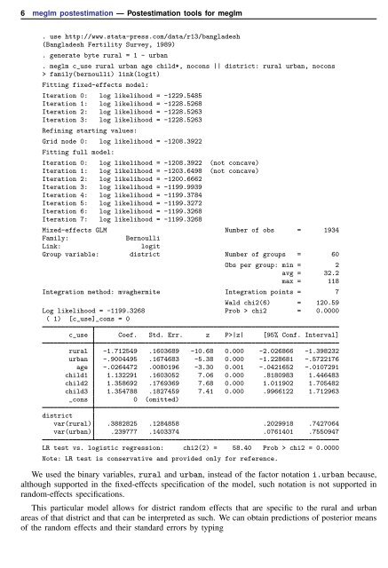
6 <strong>meglm</strong> <strong>postestimation</strong> — Postestimation tools for <strong>meglm</strong><br />
. use http://www.stata-press.com/data/r13/bangladesh<br />
(Bangladesh Fertility Survey, 1989)<br />
. generate byte rural = 1 - urban<br />
. <strong>meglm</strong> c_use rural urban age child*, nocons || district: rural urban, nocons<br />
> family(bernoulli) link(logit)<br />
Fitting fixed-effects model:<br />
Iteration 0: log likelihood = -1229.5485<br />
Iteration 1: log likelihood = -1228.5268<br />
Iteration 2: log likelihood = -1228.5263<br />
Iteration 3: log likelihood = -1228.5263<br />
Refining starting values:<br />
Grid node 0: log likelihood = -1208.3922<br />
Fitting full model:<br />
Iteration 0: log likelihood = -1208.3922 (not concave)<br />
Iteration 1: log likelihood = -1203.6498 (not concave)<br />
Iteration 2: log likelihood = -1200.6662<br />
Iteration 3: log likelihood = -1199.9939<br />
Iteration 4: log likelihood = -1199.3784<br />
Iteration 5: log likelihood = -1199.3272<br />
Iteration 6: log likelihood = -1199.3268<br />
Iteration 7: log likelihood = -1199.3268<br />
Mixed-effects GLM Number of obs = 1934<br />
Family:<br />
Bernoulli<br />
Link:<br />
logit<br />
Group variable: district Number of groups = 60<br />
Obs per group: min = 2<br />
avg = 32.2<br />
max = 118<br />
Integration method: mvaghermite Integration points = 7<br />
Wald chi2(6) = 120.59<br />
Log likelihood = -1199.3268 Prob > chi2 = 0.0000<br />
( 1) [c_use]_cons = 0<br />
c_use Coef. Std. Err. z P>|z| [95% Conf. Interval]<br />
rural -1.712549 .1603689 -10.68 0.000 -2.026866 -1.398232<br />
urban -.9004495 .1674683 -5.38 0.000 -1.228681 -.5722176<br />
age -.0264472 .0080196 -3.30 0.001 -.0421652 -.0107291<br />
child1 1.132291 .1603052 7.06 0.000 .8180983 1.446483<br />
child2 1.358692 .1769369 7.68 0.000 1.011902 1.705482<br />
child3 1.354788 .1827459 7.41 0.000 .9966122 1.712963<br />
_cons 0 (omitted)<br />
district<br />
var(rural) .3882825 .1284858 .2029918 .7427064<br />
var(urban) .239777 .1403374 .0761401 .7550947<br />
LR test vs. logistic regression: chi2(2) = 58.40 Prob > chi2 = 0.0000<br />
Note: LR test is conservative and provided only for reference.<br />
We used the binary variables, rural and urban, instead of the factor notation i.urban because,<br />
although supported in the fixed-effects specification of the model, such notation is not supported in<br />
random-effects specifications.<br />
This particular model allows for district random effects that are specific to the rural and urban<br />
areas of that district and that can be interpreted as such. We can obtain predictions of posterior means<br />
of the random effects and their standard errors by typing


