meglm postestimation - Stata

More documents

Recommendations

Info

8 meglm postestimation — Postestimation tools for meglm Had we imposed an unstructured covariance structure in our model, the estimated posterior modes and posterior means in the cases in question would not be exactly 0 because of the correlation between urban and rural effects. For instance, if a district has no urban areas, it can still yield a nonzero (albeit small) random-effects estimate for a nonexistent urban area because of the correlation with its rural counterpart; see example 1 of [ME] meqrlogit postestimation for details. Example 2 Continuing with the model from example 1, we can obtain predicted probabilities, and unless we specify the fixedonly option, these predictions will incorporate the estimated subject-specific random effects ũ j . . predict pr, pr (predictions based on fixed effects and posterior means of random effects) (using 7 quadrature points) The predicted probabilities for observation i in cluster j are obtained by applying the inverse link function to the linear predictor, ̂p ij = g −1 (x ij ̂β + zij ũ j ); see Methods and formulas for details. By default, the calculation uses posterior means for ũ j unless you specify the modes option, in which case the calculation uses posterior modes for ũ j . . 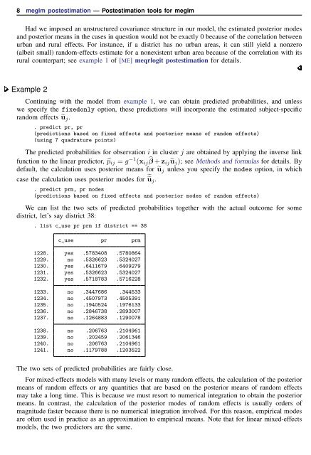predict prm, pr modes (predictions based on fixed effects and posterior modes of random effects) We can list the two sets of predicted probabilities together with the actual outcome for some district, let’s say district 38: . list c_use pr prm if district == 38 c_use pr prm 1228. yes .5783408 .5780864 1229. no .5326623 .5324027 1230. yes .6411679 .6409279 1231. yes .5326623 .5324027 1232. yes .5718783 .5716228 1233. no .3447686 .344533 1234. no .4507973 .4505391 1235. no .1940524 .1976133 1236. no .2846738 .2893007 1237. no .1264883 .1290078 1238. no .206763 .2104961 1239. no .202459 .2061346 1240. no .206763 .2104961 1241. no .1179788 .1203522 The two sets of predicted probabilities are fairly close. For mixed-effects models with many levels or many random effects, the calculation of the posterior means of random effects or any quantities that are based on the posterior means of random effects may take a long time. This is because we must resort to numerical integration to obtain the posterior means. In contrast, the calculation of the posterior modes of random effects is usually orders of magnitude faster because there is no numerical integration involved. For this reason, empirical modes are often used in practice as an approximation to empirical means. Note that for linear mixed-effects models, the two predictors are the same.
meglm postestimation — Postestimation tools for meglm 9 We can compare the observed values with the predicted values by constructing a classification table. Defining success as ŷ ij = 1 if ̂p ij > 0.5 and defining ŷ ij = 0 otherwise, we obtain the following table. . gen p_use = pr > .5 . label var p_use "Predicted outcome" . tab2 c_use p_use, row -> tabulation of c_use by p_use Key frequency row percentage Use contracept Predicted outcome ion 0 1 Total no 991 184 1,175 84.34 15.66 100.00 yes 423 336 759 55.73 44.27 100.00 Total 1,414 520 1,934 73.11 26.89 100.00 The model correctly classified 84% of women who did not use contraceptives but only 44% of women who did. In the next example, we will look at some residual diagnostics. Technical note Out-of-sample predictions are permitted after meglm, but if these predictions involve estimated random effects, the integrity of the estimation data must be preserved. If the estimation data have changed since the model was fit, predict will be unable to obtain predicted random effects that are appropriate for the fitted model and will give an error. Thus to obtain out-of-sample predictions that contain random-effects terms, be sure that the data for these predictions are in observations that augment the estimation data. Example 3 Continuing our discussion from example 2, here we look at residual diagnostics. meglm offers three kinds of predicted residuals for nonlinear responses—Pearson, Anscombe, and deviance. Of the three, Anscombe residuals are designed to be approximately normally distributed; thus we can check for outliers by plotting Anscombe residuals against observation numbers and seeing which residuals are greater than 2 in absolute value.
Page 1 and 2: Title stata.com meglm postestimatio
Page 3 and 4: meglm postestimation — Postestima
Page 7: meglm postestimation — Postestima
Page 17: meglm postestimation — Postestima

meglm postestimation - Stata

Create successful ePaper yourself

Delete template?

Save as template?