

qreg - Stata
qreg - Stata
qreg - Stata

You also want an ePaper? Increase the reach of your titles
YUMPU automatically turns print PDFs into web optimized ePapers that Google loves.
Title<br />
stata.com<br />
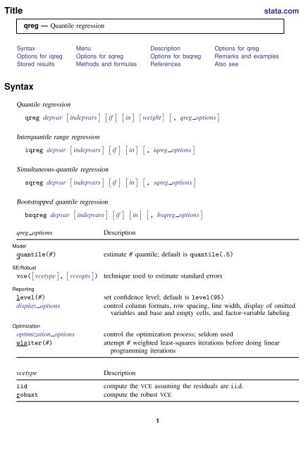
<strong>qreg</strong> — Quantile regression<br />
Syntax Menu Description Options for <strong>qreg</strong><br />
Options for i<strong>qreg</strong> Options for s<strong>qreg</strong> Options for bs<strong>qreg</strong> Remarks and examples<br />
Stored results Methods and formulas References Also see<br />
Syntax<br />
Quantile regression<br />
<strong>qreg</strong> depvar [ indepvars ] [ if ] [ in ] [ weight ] [ , <strong>qreg</strong> options ]<br />
Interquantile range regression<br />
i<strong>qreg</strong> depvar [ indepvars ] [ if ] [ in ] [ , i<strong>qreg</strong> options ]<br />
Simultaneous-quantile regression<br />
s<strong>qreg</strong> depvar [ indepvars ] [ if ] [ in ] [ , s<strong>qreg</strong> options ]<br />
Bootstrapped quantile regression<br />
bs<strong>qreg</strong> depvar [ indepvars ] [ if ] [ in ] [ , bs<strong>qreg</strong> options ]<br />
<strong>qreg</strong> options<br />
Model<br />
quantile(#)<br />
SE/Robust<br />
vce( [ vcetype ] , [ vceopts ] )<br />
Reporting<br />
level(#)<br />
display options<br />
Optimization<br />
optimization options<br />
wlsiter(#)<br />
Description<br />
estimate # quantile; default is quantile(.5)<br />
technique used to estimate standard errors<br />
set confidence level; default is level(95)<br />
control column formats, row spacing, line width, display of omitted<br />
variables and base and empty cells, and factor-variable labeling<br />
control the optimization process; seldom used<br />
attempt # weighted least-squares iterations before doing linear<br />
programming iterations<br />
vcetype<br />
iid<br />
robust<br />
Description<br />
compute the VCE assuming the residuals are i.i.d.<br />
compute the robust VCE<br />
1
2 <strong>qreg</strong> — Quantile regression<br />
vceopts<br />
denmethod<br />
bwidth<br />
Description<br />
nonparametric density estimation technique<br />
bandwidth method used by the density estimator<br />
denmethod<br />
fitted<br />
residual<br />
kernel [ (kernel) ]<br />
Description<br />
use the empirical quantile function using fitted values; the default<br />
use the empirical residual quantile function<br />
use a nonparametric kernel density estimator; default is<br />
epanechnikov<br />
bwidth<br />
hsheather<br />
bofinger<br />
chamberlain<br />
Description<br />
Hall–Sheather’s bandwidth; the default<br />
Bofinger’s bandwidth<br />
Chamberlain’s bandwidth<br />
kernel<br />
epanechnikov<br />
epan2<br />
biweight<br />
cosine<br />
gaussian<br />
parzen<br />
rectangle<br />
triangle<br />
Description<br />
Epanechnikov kernel function; the default<br />
alternative Epanechnikov kernel function<br />
biweight kernel function<br />
cosine trace kernel function<br />
Gaussian kernel function<br />
Parzen kernel function<br />
rectangle kernel function<br />
triangle kernel function<br />
i<strong>qreg</strong> options<br />
Description<br />
Model<br />
quantiles(# #) interquantile range; default is quantiles(.25 .75)<br />
reps(#)<br />
perform # bootstrap replications; default is reps(20)<br />
Reporting<br />
level(#)<br />
nodots<br />
display options<br />
set confidence level; default is level(95)<br />
suppress display of the replication dots<br />
control column formats, row spacing, line width, display of omitted<br />
variables and base and empty cells, and factor-variable labeling
<strong>qreg</strong> — Quantile regression 3<br />
s<strong>qreg</strong> options<br />
Description<br />
Model<br />
quantiles(# [ # [ # . . . ] ] ) estimate # quantiles; default is quantiles(.5)<br />
reps(#)<br />
perform # bootstrap replications; default is reps(20)<br />
Reporting<br />
level(#)<br />
nodots<br />
display options<br />
set confidence level; default is level(95)<br />
suppress display of the replication dots<br />
control column formats, row spacing, line width, display of omitted<br />
variables and base and empty cells, and factor-variable labeling<br />
bs<strong>qreg</strong> options<br />
Model<br />
quantile(#)<br />
reps(#)<br />
Reporting<br />
level(#)<br />
display options<br />
Description<br />
estimate # quantile; default is quantile(.5)<br />
perform # bootstrap replications; default is reps(20)<br />
set confidence level; default is level(95)<br />
control column formats, row spacing, line width, display of omitted<br />
variables and base and empty cells, and factor-variable labeling<br />
indepvars may contain factor variables; see [U] 11.4.3 Factor variables.<br />
by, mi estimate, rolling, and statsby, are allowed by <strong>qreg</strong>, i<strong>qreg</strong>, s<strong>qreg</strong>, and bs<strong>qreg</strong>; mfp, nestreg, and<br />
stepwise are allowed only with <strong>qreg</strong>; see [U] 11.1.10 Prefix commands.<br />
<strong>qreg</strong> allows fweights, iweights, and pweights; see [U] 11.1.6 weight.<br />
See [U] 20 Estimation and postestimation commands for more capabilities of estimation commands.<br />
Menu<br />
<strong>qreg</strong><br />
Statistics > Nonparametric analysis > Quantile regression<br />
i<strong>qreg</strong><br />
Statistics > Nonparametric analysis > Interquantile regression<br />
s<strong>qreg</strong><br />
Statistics > Nonparametric analysis > Simultaneous-quantile regression<br />
bs<strong>qreg</strong><br />
Statistics > Nonparametric analysis > Bootstrapped quantile regression<br />
Description<br />
<strong>qreg</strong> fits quantile (including median) regression models, also known as least–absolute-value models<br />
(LAV or MAD) and minimum L1-norm models. The quantile regression models fit by <strong>qreg</strong> express<br />
the quantiles of the conditional distribution as linear functions of the independent variables.
4 <strong>qreg</strong> — Quantile regression<br />
i<strong>qreg</strong> estimates interquantile range regressions, regressions of the difference in quantiles. The<br />
estimated variance–covariance matrix of the estimators (VCE) is obtained via bootstrapping.<br />
s<strong>qreg</strong> estimates simultaneous-quantile regression. It produces the same coefficients as <strong>qreg</strong> for<br />
each quantile. Reported standard errors will be similar, but s<strong>qreg</strong> obtains an estimate of the VCE<br />
via bootstrapping, and the VCE includes between-quantile blocks. Thus you can test and construct<br />
confidence intervals comparing coefficients describing different quantiles.<br />
bs<strong>qreg</strong> is equivalent to s<strong>qreg</strong> with one quantile.<br />
Options for <strong>qreg</strong><br />
✄<br />
✄<br />
✄<br />
Model<br />
<br />
quantile(#) specifies the quantile to be estimated and should be a number between 0 and 1, exclusive.<br />
Numbers larger than 1 are interpreted as percentages. The default value of 0.5 corresponds to the<br />
median.<br />
✄<br />
SE/Robust<br />
<br />
vce( [ vcetype ] , [ vceopts ] ) specifies the type of VCE to compute and the density estimation method<br />
to use in computing the VCE.<br />
vcetype specifies the type of VCE to compute. Available types are iid and robust.<br />
vce(iid), the default, computes the VCE under the assumption that the residuals are independent<br />
and identically distributed (i.i.d.).<br />
vce(robust) computes the robust VCE under the assumption that the residual density is continuous<br />
and bounded away from 0 and infinity at the specified quantile(); see Koenker (2005,<br />
sec. 4.2).<br />
vceopts consists of available denmethod and bwidth options.<br />
denmethod specifies the method to use for the nonparametric density estimator. Available<br />
methods are fitted, residual, or kernel [ (kernel) ] , where the optional kernel must be<br />
one of the kernel choices listed below.<br />
fitted and residual specify that the nonparametric density estimator use some of the<br />
structure imposed by quantile regression. The default fitted uses a function of the fitted<br />
values and residual uses a function of the residuals. vce(robust, residual) is not<br />
allowed.<br />
kernel() specifies that the nonparametric density estimator use a kernel method. The<br />
available kernel functions are epanechnikov, epan2, biweight, cosine, gaussian,<br />
parzen, rectangle, and triangle. The default is epanechnikov. See [R] kdensity<br />
for the kernel function forms.<br />
bwidth specifies the bandwidth method to use by the nonparametric density estimator. Available<br />
methods are hsheather for the Hall–Sheather bandwidth, bofinger for the Bofinger<br />
bandwidth, and chamberlain for the Chamberlain bandwidth.<br />
See Koenker (2005, sec. 3.4 and 4.10) for a description of the sparsity estimation techniques<br />
and the Hall–Sheather and Bofinger bandwidth formulas. See Chamberlain (1994, eq. 2.2) for the<br />
Chamberlain bandwidth.<br />
✄ <br />
✄ Reporting<br />
level(#); see [R] estimation options.
<strong>qreg</strong> — Quantile regression 5<br />
✄<br />
display options: noomitted, vsquish, noemptycells, baselevels, allbaselevels, nofvlabel,<br />
fvwrap(#), fvwrapon(style), cformat(% fmt), pformat(% fmt), sformat(% fmt), and<br />
nolstretch; see [R] estimation options.<br />
✄<br />
Optimization<br />
<br />
optimization options: iterate(#), [ no ] log, trace. iterate() specifies the maximum number of<br />
iterations; log/nolog specifies whether to show the iteration log; and trace specifies that the<br />
iteration log should include the current parameter vector. These options are seldom used.<br />
wlsiter(#) specifies the number of weighted least-squares iterations that will be attempted before<br />
the linear programming iterations are started. The default value is 1. If there are convergence<br />
problems, increasing this number should help.<br />
Options for i<strong>qreg</strong><br />
✄<br />
✄<br />
Model<br />
<br />
quantiles(# #) specifies the quantiles to be compared. The first number must be less than the<br />
second, and both should be between 0 and 1, exclusive. Numbers larger than 1 are interpreted as<br />
percentages. Not specifying this option is equivalent to specifying quantiles(.25 .75), meaning<br />
the interquantile range.<br />
reps(#) specifies the number of bootstrap replications to be used to obtain an estimate of the<br />
variance–covariance matrix of the estimators (standard errors). reps(20) is the default and is<br />
arguably too small. reps(100) would perform 100 bootstrap replications. reps(1000) would<br />
perform 1,000 replications.<br />
✄ <br />
✄ Reporting<br />
level(#); see [R] estimation options.<br />
nodots suppresses display of the replication dots.<br />
display options: noomitted, vsquish, noemptycells, baselevels, allbaselevels, nofvlabel,<br />
fvwrap(#), fvwrapon(style), cformat(% fmt), pformat(% fmt), sformat(% fmt), and<br />
nolstretch; see [R] estimation options.<br />
<br />
<br />
<br />
Options for s<strong>qreg</strong><br />
✄<br />
✄<br />
Model<br />
<br />
quantiles(# [ # [ # . . . ] ] ) specifies the quantiles to be estimated and should contain numbers<br />
between 0 and 1, exclusive. Numbers larger than 1 are interpreted as percentages. The default<br />
value of 0.5 corresponds to the median.<br />
reps(#) specifies the number of bootstrap replications to be used to obtain an estimate of the<br />
variance–covariance matrix of the estimators (standard errors). reps(20) is the default and is<br />
arguably too small. reps(100) would perform 100 bootstrap replications. reps(1000) would<br />
perform 1,000 replications.<br />
✄ <br />
✄ Reporting<br />
level(#); see [R] estimation options.<br />
nodots suppresses display of the replication dots.
6 <strong>qreg</strong> — Quantile regression<br />
display options: noomitted, vsquish, noemptycells, baselevels, allbaselevels, nofvlabel,<br />
fvwrap(#), fvwrapon(style), cformat(% fmt), pformat(% fmt), sformat(% fmt), and<br />
nolstretch; see [R] estimation options.<br />
Options for bs<strong>qreg</strong><br />
✄<br />
✄<br />
Model<br />
<br />
quantile(#) specifies the quantile to be estimated and should be a number between 0 and 1, exclusive.<br />
Numbers larger than 1 are interpreted as percentages. The default value of 0.5 corresponds to the<br />
median.<br />
reps(#) specifies the number of bootstrap replications to be used to obtain an estimate of the<br />
variance–covariance matrix of the estimators (standard errors). reps(20) is the default and is<br />
arguably too small. reps(100) would perform 100 bootstrap replications. reps(1000) would<br />
perform 1,000 replications.<br />
✄ <br />
✄ Reporting<br />
level(#); see [R] estimation options.<br />
display options: noomitted, vsquish, noemptycells, baselevels, allbaselevels, nofvlabel,<br />
fvwrap(#), fvwrapon(style), cformat(% fmt), pformat(% fmt), sformat(% fmt), and<br />
nolstretch; see [R] estimation options.<br />
<br />
<br />
Remarks and examples<br />
Remarks are presented under the following headings:<br />
Median regression<br />
Quantile regression<br />
Estimated standard errors<br />
Interquantile and simultaneous-quantile regression<br />
What are the parameters?<br />
stata.com<br />
Median regression<br />
<strong>qreg</strong> fits quantile regression models. The default form is median regression, where the objective is<br />
to estimate the median of the dependent variable, conditional on the values of the independent variables.<br />
This method is similar to ordinary regression, where the objective is to estimate the conditional mean<br />
of the dependent variable. Simply put, median regression finds a line through the data that minimizes<br />
the sum of the absolute residuals rather than the sum of the squares of the residuals, as in ordinary<br />
regression. Equivalently, median regression expresses the median of the conditional distribution of<br />
the dependent variable as a linear function of the conditioning (independent) variables. Cameron and<br />
Trivedi (2010, chap. 7) provide a nice introduction to quantile regression using <strong>Stata</strong>.
<strong>qreg</strong> — Quantile regression 7<br />
Example 1: Estimating the conditional median<br />
Consider a two-group experimental design with 5 observations per group:<br />
. use http://www.stata-press.com/data/r13/twogrp<br />
. list<br />
x<br />
y<br />
1. 0 0<br />
2. 0 1<br />
3. 0 3<br />
4. 0 4<br />
5. 0 95<br />
6. 1 14<br />
7. 1 19<br />
8. 1 20<br />
9. 1 22<br />
10. 1 23<br />
. <strong>qreg</strong> y x<br />
Iteration 1: WLS sum of weighted deviations = 121.88268<br />
Iteration 1: sum of abs. weighted deviations = 111<br />
Iteration 2: sum of abs. weighted deviations = 110<br />
Median regression Number of obs = 10<br />
Raw sum of deviations 157 (about 14)<br />
Min sum of deviations 110 Pseudo R2 = 0.2994<br />
y Coef. Std. Err. t P>|t| [95% Conf. Interval]<br />
x 17 18.23213 0.93 0.378 -25.04338 59.04338<br />
_cons 3 12.89207 0.23 0.822 -26.72916 32.72916<br />
We have estimated the equation<br />
y median = 3 + 17 x<br />
We look back at our data. x takes on the values 0 and 1, so the median for the x = 0 group is 3,<br />
whereas for x = 1 it is 3 + 17 = 20. The output reports that the raw sum of absolute deviations about<br />
14 is 157; that is, the sum of |y − 14| is 157. Fourteen is the unconditional median of y, although<br />
in these data, any value between 14 and 19 could also be considered an unconditional median (we<br />
have an even number of observations, so the median is bracketed by those two values). In any case,<br />
the raw sum of deviations of y about the median would be the same no matter what number we<br />
choose between 14 and 19. (With a “median” of 14, the raw sum of deviations is 157. Now think<br />
of choosing a slightly larger number for the median and recalculating the sum. Half the observations<br />
will have larger negative residuals, but the other half will have smaller positive residuals, resulting in<br />
no net change.)<br />
We turn now to the actual estimated equation. The sum of the absolute deviations about the<br />
solution y median = 3 + 17x is 110. The pseudo-R 2 is calculated as 1 − 110/157 ≈ 0.2994. This<br />
result is based on the idea that the median regression is the maximum likelihood estimate for the<br />
double-exponential distribution.
8 <strong>qreg</strong> — Quantile regression<br />
Technical note<br />
<strong>qreg</strong> is an alternative to regular regression or robust regression—see [R] regress and [R] rreg.<br />
Let’s compare the results:<br />
. regress y x<br />
Source SS df MS Number of obs = 10<br />
F( 1, 8) = 0.00<br />
Model 2.5 1 2.5 Prob > F = 0.9586<br />
Residual 6978.4 8 872.3 R-squared = 0.0004<br />
Adj R-squared = -0.1246<br />
Total 6980.9 9 775.655556 Root MSE = 29.535<br />
y Coef. Std. Err. t P>|t| [95% Conf. Interval]<br />
x -1 18.6794 -0.05 0.959 -44.07477 42.07477<br />
_cons 20.6 13.20833 1.56 0.157 -9.858465 51.05847<br />
Unlike <strong>qreg</strong>, regress fits ordinary linear regression and is concerned with predicting the mean rather<br />
than the median, so both results are, in a technical sense, correct. Putting aside those technicalities,<br />
however, we tend to use either regression to describe the central tendency of the data, of which the<br />
mean is one measure and the median another. Thus we can ask, “which method better describes the<br />
central tendency of these data?”<br />
Means—and therefore ordinary linear regression—are sensitive to outliers, and our data were<br />
purposely designed to contain two such outliers: 95 for x = 0 and 14 for x = 1. These two outliers<br />
dominated the ordinary regression and produced results that do not reflect the central tendency<br />
well—you are invited to enter the data and graph y against x.<br />
Robust regression attempts to correct the outlier-sensitivity deficiency in ordinary regression:<br />
. rreg y x, genwt(wt)<br />
Huber iteration 1: maximum difference in weights = .7311828<br />
Huber iteration 2: maximum difference in weights = .17695779<br />
Huber iteration 3: maximum difference in weights = .03149585<br />
Biweight iteration 4: maximum difference in weights = .1979335<br />
Biweight iteration 5: maximum difference in weights = .23332905<br />
Biweight iteration 6: maximum difference in weights = .09960067<br />
Biweight iteration 7: maximum difference in weights = .02691458<br />
Biweight iteration 8: maximum difference in weights = .0009113<br />
Robust regression Number of obs = 10<br />
F( 1, 8) = 80.63<br />
Prob > F = 0.0000<br />
y Coef. Std. Err. t P>|t| [95% Conf. Interval]<br />
x 18.16597 2.023114 8.98 0.000 13.50066 22.83128<br />
_cons 2.000003 1.430558 1.40 0.200 -1.298869 5.298875<br />
Here rreg discarded the first outlier completely. (We know this because we included the genwt()<br />
option on rreg and, after fitting the robust regression, examined the weights.) For the other “outlier”,<br />
rreg produced a weight of 0.47.<br />
In any case, the answers produced by <strong>qreg</strong> and rreg to describe the central tendency are similar,<br />
but the standard errors are different. In general, robust regression will have smaller standard errors<br />
because it is not as sensitive to the exact placement of observations near the median. You are welcome<br />
to try removing the first outlier in the <strong>qreg</strong> estimation to observe an improvement in the standard<br />
errors by typing
<strong>qreg</strong> — Quantile regression 9<br />
. <strong>qreg</strong> y x if _n!=5<br />
Also, some authors (Rousseeuw and Leroy 1987, 11) have noted that quantile regression, unlike the<br />
unconditional median, may be sensitive to even one outlier if its leverage is high enough. Rousseeuw<br />
and Leroy (1987) discuss estimators that are more robust to perturbations to the data than either mean<br />
regression or quantile regression.<br />
In the end, quantile regression may be more useful for the interpretation of the parameters that it<br />
estimates than for its robustness to perturbations to the data.<br />
Example 2: Median regression<br />
Let’s now consider a less artificial example using the automobile data described in [U] 1.2.2 Example<br />
datasets. Using median regression, we will regress each car’s price on its weight and length and<br />
whether it is of foreign manufacture:<br />
. use http://www.stata-press.com/data/r13/auto, clear<br />
(1978 Automobile Data)<br />
. <strong>qreg</strong> price weight length foreign<br />
Iteration 1: WLS sum of weighted deviations = 112795.66<br />
Iteration 1: sum of abs. weighted deviations = 111901<br />
Iteration 2: sum of abs. weighted deviations = 110529.43<br />
Iteration 3: sum of abs. weighted deviations = 109524.57<br />
Iteration 4: sum of abs. weighted deviations = 109468.3<br />
Iteration 5: sum of abs. weighted deviations = 109105.27<br />
note: alternate solutions exist<br />
Iteration 6: sum of abs. weighted deviations = 108931.02<br />
Iteration 7: sum of abs. weighted deviations = 108887.4<br />
Iteration 8: sum of abs. weighted deviations = 108822.59<br />
Median regression Number of obs = 74<br />
Raw sum of deviations 142205 (about 4934)<br />
Min sum of deviations 108822.6 Pseudo R2 = 0.2347<br />
price Coef. Std. Err. t P>|t| [95% Conf. Interval]<br />
weight 3.933588 1.328718 2.96 0.004 1.283543 6.583632<br />
length -41.25191 45.46469 -0.91 0.367 -131.9284 49.42456<br />
foreign 3377.771 885.4198 3.81 0.000 1611.857 5143.685<br />
_cons 344.6489 5182.394 0.07 0.947 -9991.31 10680.61<br />
The estimated equation is<br />
price median = 3.93 weight − 41.25 length + 3377.8 foreign + 344.65<br />
The output may be interpreted in the same way as linear regression output; see [R] regress. The<br />
variables weight and foreign are significant, but length is not significant. The median price of<br />
the cars in these data is $4,934. This value is a median (one of the two center observations), not the<br />
median, which would typically be defined as the midpoint of the two center observations.
10 <strong>qreg</strong> — Quantile regression<br />
Quantile regression<br />
Quantile regression is similar to median regression in that it estimates an equation expressing a<br />
quantile of the conditional distribution, albeit one that generally differs from the 0.5 quantile that is<br />
the median. For example, specifying quantile(.25) estimates the parameters that describe the 25th<br />
percentile (first quartile) of the conditional distribution.<br />
Quantile regression allows for effects of the independent variables to differ over the quantiles. For<br />
example, Chamberlain (1994) finds that union membership has a larger effect on the lower quantiles<br />
than on the higher quantiles of the conditional distribution of U.S. wages. That the effects of the<br />
independent variables may vary over quantiles of the conditional distribution is an important advantage<br />
of quantile regression over mean regression.<br />
Example 3: Estimating quantiles other than the median<br />
Returning to real data, the equation for the 25th percentile of price conditional on weight,<br />
length, and foreign in our automobile data is<br />
. use http://www.stata-press.com/data/r13/auto<br />
(1978 Automobile Data)<br />
. <strong>qreg</strong> price weight length foreign, quantile(.25)<br />
Iteration 1: WLS sum of weighted deviations = 98938.47<br />
Iteration 1: sum of abs. weighted deviations = 99457.766<br />
Iteration 2: sum of abs. weighted deviations = 91339.779<br />
Iteration 3: sum of abs. weighted deviations = 86833.291<br />
Iteration 4: sum of abs. weighted deviations = 83894.441<br />
Iteration 5: sum of abs. weighted deviations = 82186.049<br />
Iteration 6: sum of abs. weighted deviations = 75246.848<br />
Iteration 7: sum of abs. weighted deviations = 71442.907<br />
Iteration 8: sum of abs. weighted deviations = 70452.616<br />
Iteration 9: sum of abs. weighted deviations = 69646.639<br />
Iteration 10: sum of abs. weighted deviations = 69603.554<br />
.25 Quantile regression Number of obs = 74<br />
Raw sum of deviations 83825.5 (about 4187)<br />
Min sum of deviations 69603.55 Pseudo R2 = 0.1697<br />
price Coef. Std. Err. t P>|t| [95% Conf. Interval]<br />
weight 1.831789 .6328903 2.89 0.005 .5695289 3.094049<br />
length 2.84556 21.65558 0.13 0.896 -40.34514 46.03626<br />
foreign 2209.925 421.7401 5.24 0.000 1368.791 3051.059<br />
_cons -1879.775 2468.46 -0.76 0.449 -6802.963 3043.413<br />
Compared with our previous median regression, the coefficient on length now has a positive sign,<br />
and the coefficients on foreign and weight are reduced. The actual lower quantile is $4,187,<br />
substantially less than the median $4,934.
<strong>qreg</strong> — Quantile regression 11<br />
We can also estimate the upper quartile as a function of the same three variables:<br />
. <strong>qreg</strong> price weight length foreign, quantile(.75)<br />
Iteration 1: WLS sum of weighted deviations = 110931.48<br />
Iteration 1: sum of abs. weighted deviations = 111305.91<br />
Iteration 2: sum of abs. weighted deviations = 105989.57<br />
Iteration 3: sum of abs. weighted deviations = 100378.89<br />
Iteration 4: sum of abs. weighted deviations = 99796.49<br />
Iteration 5: sum of abs. weighted deviations = 98796.212<br />
Iteration 6: sum of abs. weighted deviations = 98483.669<br />
Iteration 7: sum of abs. weighted deviations = 98395.935<br />
.75 Quantile regression Number of obs = 74<br />
Raw sum of deviations 159721.5 (about 6342)<br />
Min sum of deviations 98395.94 Pseudo R2 = 0.3840<br />
price Coef. Std. Err. t P>|t| [95% Conf. Interval]<br />
weight 9.22291 1.785767 5.16 0.000 5.66131 12.78451<br />
length -220.7833 61.10352 -3.61 0.001 -342.6504 -98.91616<br />
foreign 3595.133 1189.984 3.02 0.004 1221.785 5968.482<br />
_cons 20242.9 6965.02 2.91 0.005 6351.61 34134.2<br />
This result tells a different story: weight is much more important, and length is now significant—with<br />
a negative coefficient! The prices of high-priced cars seem to be determined by factors different from<br />
those affecting the prices of low-priced cars.<br />
Technical note<br />
One explanation for having substantially different regression functions for different quantiles is<br />
that the data are heteroskedastic, as we will demonstrate below. The following statements create a<br />
sharply heteroskedastic set of data:<br />
. drop _all<br />
. set obs 10000<br />
obs was 0, now 10000<br />
. set seed 50550<br />
. gen x = .1 + .9 * runiform()<br />
. gen y = x * runiform()^2
12 <strong>qreg</strong> — Quantile regression<br />
Let’s now fit the regressions for the 5th and 95th quantiles:<br />
. <strong>qreg</strong> y x, quantile(.05)<br />
Iteration 1: WLS sum of weighted deviations = 1080.7273<br />
Iteration 1: sum of abs. weighted deviations = 1078.3192<br />
Iteration 2: sum of abs. weighted deviations = 282.73545<br />
Iteration 3: sum of abs. weighted deviations = 182.46921<br />
Iteration 4: sum of abs. weighted deviations = 182.25456<br />
Iteration 5: sum of abs. weighted deviations = 182.2527<br />
Iteration 6: sum of abs. weighted deviations = 182.25247<br />
Iteration 7: sum of abs. weighted deviations = 182.25246<br />
Iteration 8: sum of abs. weighted deviations = 182.25245<br />
Iteration 9: sum of abs. weighted deviations = 182.25244<br />
.05 Quantile regression Number of obs = 10000<br />
Raw sum of deviations 182.357 (about .0009234)<br />
Min sum of deviations 182.2524 Pseudo R2 = 0.0006<br />
y Coef. Std. Err. t P>|t| [95% Conf. Interval]<br />
x .002601 .0004576 5.68 0.000 .001704 .003498<br />
_cons -.0001393 .0002782 -0.50 0.617 -.0006846 .000406<br />
. <strong>qreg</strong> y x, quantile(.95)<br />
Iteration 1: WLS sum of weighted deviations = 1237.5569<br />
Iteration 1: sum of abs. weighted deviations = 1238.0014<br />
Iteration 2: sum of abs. weighted deviations = 456.65044<br />
Iteration 3: sum of abs. weighted deviations = 338.45497<br />
Iteration 4: sum of abs. weighted deviations = 338.43897<br />
Iteration 5: sum of abs. weighted deviations = 338.4389<br />
.95 Quantile regression Number of obs = 10000<br />
Raw sum of deviations 554.6889 (about .61326343)<br />
Min sum of deviations 338.4389 Pseudo R2 = 0.3899<br />
y Coef. Std. Err. t P>|t| [95% Conf. Interval]<br />
x .8898259 .0090984 97.80 0.000 .8719912 .9076605<br />
_cons .0021514 .0055307 0.39 0.697 -.00869 .0129927<br />
The coefficient on x, in particular, differs markedly between the two estimates. For the mathematically<br />
inclined, it is not too difficult to show that the theoretical lines are y = 0.0025 x for the 5th percentile<br />
and y = 0.9025 x for the 95th, numbers in close agreement with our numerical results.<br />
The estimator for the standard errors computed by <strong>qreg</strong> assumes that the sample is independent<br />
and identically distributed (i.i.d.); see Estimated standard errors and Methods and formulas for details.<br />
Because the data are conditionally heteroskedastic, we should have used bs<strong>qreg</strong> to consistently<br />
estimate the standard errors using a bootstrap method.<br />
Estimated standard errors<br />
The variance–covariance matrix of the estimator (VCE) depends on the reciprocal of the density<br />
of the dependent variable evaluated at the quantile of interest. This function, known as the “sparsity<br />
function”, is hard to estimate.
<strong>qreg</strong> — Quantile regression 13<br />
The default method, which uses the fitted values for the predicted quantiles, generally performs<br />
well, but other methods may be preferred in larger samples. The vce() suboptions denmethod and<br />
bwidth provide other estimators of the sparsity function, the details of which are described in Methods<br />
and formulas.<br />
For models with heteroskedastic errors, option vce(robust) computes a Huber (1967) form<br />
of sandwich estimate (Koenker 2005). Alternatively, Gould (1992, 1997b) introduced generalized<br />
versions of <strong>qreg</strong> that obtain estimates of the standard errors by using bootstrap resampling (see Efron<br />
and Tibshirani [1993] or Wu [1986] for an introduction to bootstrap standard errors). The i<strong>qreg</strong>,<br />
s<strong>qreg</strong>, and bs<strong>qreg</strong> commands provide a bootstrapped estimate of the entire variance–covariance<br />
matrix of the estimators.<br />
Example 4: Obtaining robust standard errors<br />
Example 2 of <strong>qreg</strong> on real data above was a median regression of price on weight, length, and<br />
foreign using auto.dta. Suppose, after investigation, we are convinced that car price observations<br />
are not independent. We decide that standard errors robust to non-i.i.d. errors would be appropriate<br />
and use the option vce(robust).<br />
. use http://www.stata-press.com/data/r13/auto, clear<br />
(1978 Automobile Data)<br />
. <strong>qreg</strong> price weight length foreign, vce(robust)<br />
Iteration 1: WLS sum of weighted deviations = 112795.66<br />
Iteration 1: sum of abs. weighted deviations = 111901<br />
Iteration 2: sum of abs. weighted deviations = 110529.43<br />
Iteration 3: sum of abs. weighted deviations = 109524.57<br />
Iteration 4: sum of abs. weighted deviations = 109468.3<br />
Iteration 5: sum of abs. weighted deviations = 109105.27<br />
note: alternate solutions exist<br />
Iteration 6: sum of abs. weighted deviations = 108931.02<br />
Iteration 7: sum of abs. weighted deviations = 108887.4<br />
Iteration 8: sum of abs. weighted deviations = 108822.59<br />
Median regression Number of obs = 74<br />
Raw sum of deviations 142205 (about 4934)<br />
Min sum of deviations 108822.6 Pseudo R2 = 0.2347<br />
Robust<br />
price Coef. Std. Err. t P>|t| [95% Conf. Interval]<br />
weight 3.933588 1.694477 2.32 0.023 .55406 7.313116<br />
length -41.25191 51.73571 -0.80 0.428 -144.4355 61.93171<br />
foreign 3377.771 728.5115 4.64 0.000 1924.801 4830.741<br />
_cons 344.6489 5096.528 0.07 0.946 -9820.055 10509.35<br />
We see that the robust standard error for weight increases making it less significant in modifying<br />
the median automobile price. The standard error for length also increases, but the standard error<br />
for the foreign indicator decreases.
14 <strong>qreg</strong> — Quantile regression<br />
For comparison, we repeat the estimation using bootstrap standard errors:<br />
. use http://www.stata-press.com/data/r13/auto, clear<br />
(1978 Automobile Data)<br />
. set seed 1001<br />
. bs<strong>qreg</strong> price weight length foreign<br />
(fitting base model)<br />
Bootstrap replications (20)<br />
1 2 3 4 5<br />
....................<br />
Median regression, bootstrap(20) SEs Number of obs = 74<br />
Raw sum of deviations 142205 (about 4934)<br />
Min sum of deviations 108822.6 Pseudo R2 = 0.2347<br />
price Coef. Std. Err. t P>|t| [95% Conf. Interval]<br />
weight 3.933588 3.12446 1.26 0.212 -2.297951 10.16513<br />
length -41.25191 83.71267 -0.49 0.624 -208.2116 125.7077<br />
foreign 3377.771 1057.281 3.19 0.002 1269.09 5486.452<br />
_cons 344.6489 7053.301 0.05 0.961 -13722.72 14412.01<br />
The coefficient estimates are the same—indeed, they are obtained using the same technique. Only<br />
the standard errors differ. Therefore, the t statistics, significance levels, and confidence intervals also<br />
differ.<br />
Because bs<strong>qreg</strong> (as well as s<strong>qreg</strong> and i<strong>qreg</strong>) obtains standard errors by randomly resampling<br />
the data, the standard errors it produces will not be the same from run to run unless we first set the<br />
random-number seed to the same number; see [R] set seed.
<strong>qreg</strong> — Quantile regression 15<br />
By default, bs<strong>qreg</strong>, s<strong>qreg</strong>, and i<strong>qreg</strong> use 20 replications. We can control the number of<br />
replications by specifying the reps() option:<br />
. bs<strong>qreg</strong> price weight length i.foreign, reps(1000)<br />
(fitting base model)<br />
Bootstrap replications (1000)<br />
1 2 3 4 5<br />
.................................................. 50<br />
.................................................. 100<br />
.................................................. 150<br />
.................................................. 200<br />
.................................................. 250<br />
.................................................. 300<br />
.................................................. 350<br />
.................................................. 400<br />
.................................................. 450<br />
.................................................. 500<br />
.................................................. 550<br />
.................................................. 600<br />
.................................................. 650<br />
.................................................. 700<br />
.................................................. 750<br />
.................................................. 800<br />
.................................................. 850<br />
.................................................. 900<br />
.................................................. 950<br />
.................................................. 1000<br />
Median regression, bootstrap(1000) SEs Number of obs = 74<br />
Raw sum of deviations 142205 (about 4934)<br />
Min sum of deviations 108822.6 Pseudo R2 = 0.2347<br />
price Coef. Std. Err. t P>|t| [95% Conf. Interval]<br />
weight 3.933588 2.659349 1.48 0.144 -1.370316 9.237492<br />
length -41.25191 69.29744 -0.60 0.554 -179.4613 96.95748<br />
foreign<br />
Foreign 3377.771 1096.197 3.08 0.003 1191.474 5564.068<br />
_cons 344.6489 5916.939 0.06 0.954 -11456.31 12145.61<br />
A comparison of the standard errors is informative.<br />
<strong>qreg</strong> bs<strong>qreg</strong> bs<strong>qreg</strong><br />
Variable <strong>qreg</strong> vce(robust) reps(20) reps(1000)<br />
weight 1.329 1.694 3.124 2.660<br />
length 45.46 51.74 83.71 69.30<br />
1.foreign 885.4 728.5 1057. 1095.<br />
cons 5182. 5096. 7053. 5917.<br />
The results shown above are typical for models with heteroskedastic errors. (Our dependent variable<br />
is price; if our model had been in terms of ln(price), the standard errors estimated by <strong>qreg</strong> and<br />
bs<strong>qreg</strong> would have been nearly identical.) Also, even for heteroskedastic errors, 20 replications is<br />
generally sufficient for hypothesis tests against 0.
16 <strong>qreg</strong> — Quantile regression<br />
Interquantile and simultaneous-quantile regression<br />
Consider a quantile regression model where the qth quantile is given by<br />
Q q (y) = a q + b q,1 x 1 + b q,2 x 2<br />
For instance, the 75th and 25th quantiles are given by<br />
The difference in the quantiles is then<br />
Q 0.75 (y) = a 0.75 + b 0.75,1 x 1 + b 0.75,2 x 2<br />
Q 0.25 (y) = a 0.25 + b 0.25,1 x 1 + b 0.25,2 x 2<br />
Q 0.75 (y) − Q 0.25 (y) = (a 0.75 − a 0.25 ) + (b 0.75,1 − b 0.25,1 )x 1 + (b 0.75,2 − b 0.25,2 )x 2<br />
<strong>qreg</strong> fits models such as Q 0.75 (y) and Q 0.25 (y). i<strong>qreg</strong> fits interquantile models, such as Q 0.75 (y)−<br />
Q 0.25 (y). The relationships of the coefficients estimated by <strong>qreg</strong> and i<strong>qreg</strong> are exactly as shown:<br />
i<strong>qreg</strong> reports coefficients that are the difference in coefficients of two <strong>qreg</strong> models, and, of course,<br />
i<strong>qreg</strong> reports the appropriate standard errors, which it obtains by bootstrapping.<br />
s<strong>qreg</strong> is like <strong>qreg</strong> in that it estimates the equations for the quantiles<br />
Q 0.75 (y) = a 0.75 + b 0.75,1 x 1 + b 0.75,2 x 2<br />
Q 0.25 (y) = a 0.25 + b 0.25,1 x 1 + b 0.25,2 x 2<br />
The coefficients it obtains are the same that would be obtained by estimating each equation separately<br />
using <strong>qreg</strong>. s<strong>qreg</strong> differs from <strong>qreg</strong> in that it estimates the equations simultaneously and obtains<br />
an estimate of the entire variance–covariance matrix of the estimators by bootstrapping. Thus you<br />
can perform hypothesis tests concerning coefficients both within and across equations.<br />
For example, to fit the above model, you could type<br />
. <strong>qreg</strong> y x1 x2, quantile(.25)<br />
. <strong>qreg</strong> y x1 x2, quantile(.75)<br />
By doing this, you would obtain estimates of the parameters, but you could not test whether<br />
b 0.25,1 = b 0.75,1 or, equivalently, b 0.75,1 − b 0.25,1 = 0. If your interest really is in the difference of<br />
coefficients, you could type<br />
. i<strong>qreg</strong> y x1 x2, quantiles(.25 .75)<br />
The “coefficients” reported would be the difference in quantile coefficients. You could also estimate<br />
both quantiles simultaneously and then test the equality of the coefficients:<br />
. s<strong>qreg</strong> y x1 x2, quantiles(.25 .75)<br />
. test [q25]x1 = [q75]x1<br />
Whether you use i<strong>qreg</strong> or s<strong>qreg</strong> makes no difference for this test. s<strong>qreg</strong>, however, because it<br />
estimates the quantiles simultaneously, allows you to test other hypotheses. i<strong>qreg</strong>, by focusing on<br />
quantile differences, presents results in a way that is easier to read.<br />
Finally, s<strong>qreg</strong> can estimate quantiles singly,<br />
. s<strong>qreg</strong> y x1 x2, quantiles(.5)<br />
and can thereby be used as a substitute for the slower bs<strong>qreg</strong>. (Gould [1997b] presents timings<br />
demonstrating that s<strong>qreg</strong> is faster than bs<strong>qreg</strong>.) s<strong>qreg</strong> can also estimate more than two quantiles<br />
simultaneously:<br />
. s<strong>qreg</strong> y x1 x2, quantiles(.25 .5 .75)
<strong>qreg</strong> — Quantile regression 17<br />
Example 5: Simultaneous quantile estimation<br />
In demonstrating <strong>qreg</strong>, we performed quantile regressions using auto.dta. We discovered that<br />
the regression of price on weight, length, and foreign produced vastly different coefficients for<br />
the 0.25, 0.5, and 0.75 quantile regressions. Here are the coefficients that we obtained:<br />
25th 50th 75th<br />
Variable percentile percentile percentile<br />
weight 1.83 3.93 9.22<br />
length 2.85 −41.25 −220.8<br />
foreign 2209.9 3377.8 3595.1<br />
cons −1879.8 344.6 20242.9<br />
All we can say, having estimated these equations separately, is that price seems to depend differently<br />
on the weight, length, and foreign variables depending on the portion of the price distribution<br />
we examine. We cannot be more precise because the estimates have been made separately. With<br />
s<strong>qreg</strong>, however, we can estimate all the effects simultaneously:<br />
. use http://www.stata-press.com/data/r13/auto, clear<br />
(1978 Automobile Data)<br />
. set seed 1001<br />
. s<strong>qreg</strong> price weight length foreign, q(.25 .5 .75) reps(100)<br />
(fitting base model)<br />
Bootstrap replications (100)<br />
1 2 3 4 5<br />
.................................................. 50<br />
.................................................. 100<br />
Simultaneous quantile regression Number of obs = 74<br />
bootstrap(100) SEs .25 Pseudo R2 = 0.1697<br />
.50 Pseudo R2 = 0.2347<br />
.75 Pseudo R2 = 0.3840<br />
Bootstrap<br />
price Coef. Std. Err. t P>|t| [95% Conf. Interval]<br />
q25<br />
q50<br />
q75<br />
weight 1.831789 1.574777 1.16 0.249 -1.309005 4.972583<br />
length 2.84556 38.63523 0.07 0.941 -74.20998 79.9011<br />
foreign 2209.925 1008.521 2.19 0.032 198.494 4221.357<br />
_cons -1879.775 3665.184 -0.51 0.610 -9189.753 5430.204<br />
weight 3.933588 2.529541 1.56 0.124 -1.111423 8.978599<br />
length -41.25191 68.62258 -0.60 0.550 -178.1153 95.61151<br />
foreign 3377.771 1017.422 3.32 0.001 1348.586 5406.956<br />
_cons 344.6489 6199.257 0.06 0.956 -12019.38 12708.68<br />
weight 9.22291 2.483676 3.71 0.000 4.269374 14.17645<br />
length -220.7833 86.17422 -2.56 0.013 -392.6524 -48.91421<br />
foreign 3595.133 1147.216 3.13 0.003 1307.083 5883.184<br />
_cons 20242.9 9414.242 2.15 0.035 1466.79 39019.02<br />
The coefficient estimates above are the same as those previously estimated, although the standard error<br />
estimates are a little different. s<strong>qreg</strong> obtains estimates of variance by bootstrapping. The important<br />
thing here, however, is that the full covariance matrix of the estimators has been estimated and stored,<br />
and thus it is now possible to perform hypothesis tests. Are the effects of weight the same at the<br />
25th and 75th percentiles?
18 <strong>qreg</strong> — Quantile regression<br />
. test [q25]weight = [q75]weight<br />
( 1) [q25]weight - [q75]weight = 0<br />
F( 1, 70) = 8.97<br />
Prob > F = 0.0038<br />
It appears that they are not. We can obtain a confidence interval for the difference by using lincom:<br />
. lincom [q75]weight-[q25]weight<br />
( 1) - [q25]weight + [q75]weight = 0<br />
price Coef. Std. Err. t P>|t| [95% Conf. Interval]<br />
(1) 7.391121 2.467548 3.00 0.004 2.469752 12.31249<br />
Indeed, we could test whether the weight and length sets of coefficients are equal at the three<br />
quantiles estimated:<br />
. quietly test [q25]weight = [q50]weight<br />
. quietly test [q25]weight = [q75]weight, accumulate<br />
. quietly test [q25]length = [q50]length, accumulate<br />
. test [q25]length = [q75]length, accumulate<br />
( 1) [q25]weight - [q50]weight = 0<br />
( 2) [q25]weight - [q75]weight = 0<br />
( 3) [q25]length - [q50]length = 0<br />
( 4) [q25]length - [q75]length = 0<br />
F( 4, 70) = 2.43<br />
Prob > F = 0.0553<br />
i<strong>qreg</strong> focuses on one quantile comparison but presents results that are more easily interpreted:<br />
. set seed 1001<br />
. i<strong>qreg</strong> price weight length foreign, q(.25 .75) reps(100) nolog<br />
.75-.25 Interquantile regression Number of obs = 74<br />
bootstrap(100) SEs .75 Pseudo R2 = 0.3840<br />
.25 Pseudo R2 = 0.1697<br />
Bootstrap<br />
price Coef. Std. Err. t P>|t| [95% Conf. Interval]<br />
weight 7.391121 2.467548 3.00 0.004 2.469752 12.31249<br />
length -223.6288 83.09868 -2.69 0.009 -389.3639 -57.89376<br />
foreign 1385.208 1193.557 1.16 0.250 -995.2672 3765.683<br />
_cons 22122.68 9009.159 2.46 0.017 4154.478 40090.88<br />
Looking only at the 0.25 and 0.75 quantiles (the interquartile range), the i<strong>qreg</strong> command output<br />
is easily interpreted. Increases in weight correspond significantly to increases in price dispersion.<br />
Increases in length correspond to decreases in price dispersion. The foreign variable does not<br />
significantly change price dispersion.<br />
Do not make too much of these results; the purpose of this example is simply to illustrate the<br />
s<strong>qreg</strong> and i<strong>qreg</strong> commands and to do so in a context that suggests why analyzing dispersion might<br />
be of interest.
<strong>qreg</strong> — Quantile regression 19<br />
lincom after s<strong>qreg</strong> produced the same t statistic for the interquartile range of weight, as did<br />
the i<strong>qreg</strong> command above. In general, they will not agree exactly because of the randomness of<br />
bootstrapping, unless the random-number seed is set to the same value before estimation (as was<br />
done here).<br />
Gould (1997a) presents simulation results showing that the coverage—the actual percentage of<br />
confidence intervals containing the true value—for i<strong>qreg</strong> is appropriate.<br />
What are the parameters?<br />
In this section, we use a specific data-generating process (DGP) to illustrate the interpretation of the<br />
parameters estimated by <strong>qreg</strong>. If simulation experiments are not intuitive to you, skip this section.<br />
In general, quantile regression parameterizes the quantiles of the distribution of y conditional on<br />
the independent variables x as xβ, where β is a vector of estimated parameters. In our example, we<br />
include a constant term and a single independent variable, and we express quantiles of the distribution<br />
of y conditional on x as β 0 + β 1 x.<br />
We use simulated data to illustrate what we mean by a conditional distribution and how to interpret<br />
the parameters β estimated by <strong>qreg</strong>. We also note how we could change our example to illustrate a<br />
DGP for which the estimator in <strong>qreg</strong> would be misspecified.<br />
We suppose that the distribution of y conditional on x has a Weibull form. If y has a Weibull<br />
distribution, the distribution function is F (y) = 1−exp{−(y/λ) k }, where the scale parameter λ > 0<br />
and the shape parameter k > 0. We can make y have a Weibull distribution function conditional on<br />
x by making the scale parameter or the shape parameter functions of x. In our example, we specify<br />
a particular DGP by supposing that λ = (1 + αx), α = 1.5, x = 1 + √ ν, and that ν has a χ 2 (1)<br />
distribution. For the moment, we leave the parameter k as is so that we can discuss how this decision<br />
relates to model specification.<br />
Plugging in for λ yields the functional form for the distribution of y conditional on x, which is<br />
known as the conditional distribution function and is denoted F (y|x). F (y|x) is the distribution for<br />
y for each given value of x.<br />
Some algebra yields that F (y|x) = 1 − exp[−{y/(1 + αx)} k ]. Letting τ = F (y|x) implies that<br />
0 ≤ τ ≤ 1, because probabilities must be between 0 and 1.<br />
To obtain the τ quantile of the distribution of y conditional on x, we solve<br />
τ = 1 − exp[−{y/(1 + αx)} k ]<br />
for y as a function of τ, x, α, and k. The solution is<br />
y = (1 + αx){− ln(1 − τ)} (1/k) (1)<br />
For any value of τ ∈ (0, 1), expression (1) gives the τ quantile of the distribution of y conditional<br />
on x. To use <strong>qreg</strong>, we must rewrite (1) as a function of x, β 0 , and β 1 . Some algebra yields that (1)<br />
can be rewritten as<br />
y = β 0 + β 1 ∗ x<br />
where β 0 = {− ln(1 − τ)} (1/k) and β 1 = α{− ln(1 − τ)} (1/k) . We can express the conditional<br />
quantiles as linear combinations of x, which is a property of the estimator implemented in <strong>qreg</strong>.
20 <strong>qreg</strong> — Quantile regression<br />
If we parameterize k as a nontrivial function of x, the conditional quantiles will not be linear<br />
in x. If the conditional quantiles cannot be represented as linear functions of x, we cannot estimate<br />
the true parameters of the DGP. This restriction illustrates the limits of the estimator implemented in<br />
<strong>qreg</strong>.<br />
We set k = 2 for our example.<br />
Conditional quantile regression allows the coefficients to change with the specified quantile. For<br />
our DGP, the coefficients β 0 and β 1 increase as τ gets larger. Substituting in for α and k yields that<br />
β 0 = √ − ln(1 − τ) and β 1 = 1.5 √ − ln(1 − τ). Table 1 presents the true values for β 0 and β 1<br />
implied by our DGP when τ ∈ {0.25, 0.5, 0.8}.<br />
Table 1: True values for β 0 and β 1<br />
τ β 0 β 1<br />
0.25 0.53636 0.80454<br />
0.5 0.8325546 1.248832<br />
0.8 1.268636 1.902954<br />
We can also use (1) to generate data from the specified distribution of y conditional on x by<br />
plugging in random uniform numbers for τ. Each random uniform number substituted in for τ in (1)<br />
yields a draw from the conditional distribution of y given x.<br />
Example 6<br />
In this example, we generate 100,000 observations from our specified DGP by substituting random<br />
uniform numbers for τ in (1), with α = 1.5, k = 2, x = 1 + √ ν, and ν coming from a χ 2 (1)<br />
distribution.<br />
We begin by executing the code that implements this method; below we discuss each line of the<br />
output produced.<br />
. clear // drop existing variables<br />
. set seed 1234571 // set random-number seed<br />
. set obs 100000 // set number of observations<br />
obs was 0, now 100000<br />
. generate double tau = runiform() // generate uniform variate<br />
. generate double x = 1 + sqrt(rchi2(1)) // generate values for x<br />
. generate double lambda = 1 + 1.5*x // lambda is 1 + alpha*x<br />
. generate double k = 2 // fix value of k<br />
. // generate random values for y<br />
. // given x<br />
. generate double y = lambda*((-ln(1-tau))^(1/k))<br />
Although the comments at the end of each line briefly describe what each line is doing, we provide<br />
a more careful description. The first line drops any variables in memory. The second sets the seed<br />
of the random-number generator so that we will always get the same sequence of random uniform<br />
numbers. The third line sets the sample size to 100,000 observations, and the fourth line reports the<br />
change in sample size.<br />
The fifth line substitutes random uniform numbers for τ. This line is the key to the algorithm.<br />
This standard method, known as inverse-probability transforms, for computing random numbers is<br />
discussed by Cameron and Trivedi (2010, 126–127), among others.
<strong>qreg</strong> — Quantile regression 21<br />
Lines 6–8 generate x, λ, and k per our specified DGP. Lines 9–11 implement (1) using the<br />
previously generated λ, x, and k.<br />
At the end, we have 100,000 observations on y and x, with y coming from the conditional<br />
distribution that we specified above.<br />
Example 7<br />
In the example below, we use <strong>qreg</strong> to estimate β 1 and β 0 , the parameters from the conditional<br />
quantile function, for the 0.5 quantile from our simulated data.<br />
. <strong>qreg</strong> y x, quantile(.5)<br />
Iteration 1: WLS sum of weighted deviations = 137951.03<br />
Iteration 1: sum of abs. weighted deviations = 137950.65<br />
Iteration 2: sum of abs. weighted deviations = 137687.92<br />
Iteration 3: sum of abs. weighted deviations = 137259.28<br />
Iteration 4: sum of abs. weighted deviations = 137252.76<br />
Iteration 5: sum of abs. weighted deviations = 137251.32<br />
Iteration 6: sum of abs. weighted deviations = 137251.31<br />
Iteration 7: sum of abs. weighted deviations = 137251.31<br />
Median regression Number of obs = 100000<br />
Raw sum of deviations 147681 (about 2.944248)<br />
Min sum of deviations 137251.3 Pseudo R2 = 0.0706<br />
y Coef. Std. Err. t P>|t| [95% Conf. Interval]<br />
x 1.228536 .0118791 103.42 0.000 1.205253 1.251819<br />
_cons .8693355 .0225288 38.59 0.000 .8251793 .9134917<br />
In the <strong>qreg</strong> output, the results for x correspond to the estimate of β 1 , and the results for cons<br />
correspond to the estimate of β 0 . The reported estimates are close to their true values of 1.248832<br />
and 0.8325546, which are given in table 1.<br />
The intuition in this example comes from the ability of <strong>qreg</strong> to recover the true parameters of<br />
our specified DGP. As we increase the number of observations in our sample size, the <strong>qreg</strong> estimates<br />
will get closer to the true values.
22 <strong>qreg</strong> — Quantile regression<br />
Example 8<br />
In the example below, we estimate the parameters of the conditional quantile function for the 0.25<br />
quantile and compare them with the true values.<br />
. <strong>qreg</strong> y x, quantile(.25)<br />
Iteration 1: WLS sum of weighted deviations = 130994.57<br />
Iteration 1: sum of abs. weighted deviations = 130984.72<br />
Iteration 2: sum of abs. weighted deviations = 120278.95<br />
Iteration 3: sum of abs. weighted deviations = 99999.586<br />
Iteration 4: sum of abs. weighted deviations = 99998.958<br />
Iteration 5: sum of abs. weighted deviations = 99998.93<br />
Iteration 6: sum of abs. weighted deviations = 99998.93<br />
.25 Quantile regression Number of obs = 100000<br />
Raw sum of deviations 104029.6 (about 1.857329)<br />
Min sum of deviations 99998.93 Pseudo R2 = 0.0387<br />
y Coef. Std. Err. t P>|t| [95% Conf. Interval]<br />
x .7844305 .0107092 73.25 0.000 .7634405 .8054204<br />
_cons .5633285 .0203102 27.74 0.000 .5235209 .6031362<br />
As above, <strong>qreg</strong> reports the estimates of β 1 and β 0 in the output table for x and cons, respectively.<br />
The reported estimates are close to their true values of 0.80454 and 0.53636, which are given in<br />
table 1. As expected, the estimates are close to their true values. Also as expected, the estimates for<br />
the 0.25 quantile are smaller than the estimates for the 0.5 quantile.
Example 9<br />
<strong>qreg</strong> — Quantile regression 23<br />
We finish this section by estimating the parameters of the conditional quantile function for the 0.8<br />
quantile and comparing them with the true values.<br />
. <strong>qreg</strong> y x, quantile(.8)<br />
Iteration 1: WLS sum of weighted deviations = 132664.6<br />
Iteration 1: sum of abs. weighted deviations = 132664.39<br />
Iteration 2: sum of abs. weighted deviations = 120153.29<br />
Iteration 3: sum of abs. weighted deviations = 105178.39<br />
Iteration 4: sum of abs. weighted deviations = 104681.92<br />
Iteration 5: sum of abs. weighted deviations = 104525.01<br />
Iteration 6: sum of abs. weighted deviations = 104498.61<br />
Iteration 7: sum of abs. weighted deviations = 104490.25<br />
Iteration 8: sum of abs. weighted deviations = 104490.21<br />
Iteration 9: sum of abs. weighted deviations = 104490.16<br />
Iteration 10: sum of abs. weighted deviations = 104490.15<br />
Iteration 11: sum of abs. weighted deviations = 104490.15<br />
Iteration 12: sum of abs. weighted deviations = 104490.15<br />
Iteration 13: sum of abs. weighted deviations = 104490.15<br />
Iteration 14: sum of abs. weighted deviations = 104490.15<br />
Iteration 15: sum of abs. weighted deviations = 104490.15<br />
.8 Quantile regression Number of obs = 100000<br />
Raw sum of deviations 120186.7 (about 4.7121822)<br />
Min sum of deviations 104490.1 Pseudo R2 = 0.1306<br />
y Coef. Std. Err. t P>|t| [95% Conf. Interval]<br />
x 1.889702 .0146895 128.64 0.000 1.860911 1.918493<br />
_cons 1.293773 .0278587 46.44 0.000 1.23917 1.348375<br />
As above, <strong>qreg</strong> reports the estimates of β 1 and β 0 in the output table for x and cons, respectively.<br />
The reported estimates are close to their true values of 1.902954 and 1.268636, which are given in<br />
table 1. As expected, the estimates are close to their true values. Also as expected, the estimates for<br />
the 0.8 quantile are larger than the estimates for the 0.5 quantile.
24 <strong>qreg</strong> — Quantile regression<br />
Stored results<br />
<strong>qreg</strong> stores the following in e():<br />
Scalars<br />
e(N)<br />
e(df m)<br />
e(df r)<br />
e(q)<br />
e(q v)<br />
e(sum adev)<br />
e(sum rdev)<br />
e(sum w)<br />
e(f r)<br />
e(sparsity)<br />
e(bwidth)<br />
e(kbwidth)<br />
e(rank)<br />
e(convcode)<br />
Macros<br />
e(cmd)<br />
e(cmdline)<br />
e(depvar)<br />
e(bwmethod)<br />
e(denmethod)<br />
e(kernel)<br />
e(wtype)<br />
e(wexp)<br />
e(vce)<br />
e(vcetype)<br />
e(properties)<br />
e(predict)<br />
e(marginsnotok)<br />
Matrices<br />
e(b)<br />
e(V)<br />
Functions<br />
e(sample)<br />
number of observations<br />
model degrees of freedom<br />
residual degrees of freedom<br />
quantile requested<br />
value of the quantile<br />
sum of absolute deviations<br />
sum of raw deviations<br />
sum of weights<br />
density estimate<br />
sparsity estimate<br />
bandwidth<br />
kernel bandwidth<br />
rank of e(V)<br />
0 if converged; otherwise, return code for why nonconvergence<br />
<strong>qreg</strong><br />
command as typed<br />
name of dependent variable<br />
bandwidth method; hsheather, bofinger, or chamberlain<br />
density estimation method; fitted, residual, or kernel<br />
kernel function<br />
weight type<br />
weight expression<br />
vcetype specified in vce()<br />
title used to label Std. Err.<br />
b V<br />
program used to implement predict<br />
predictions disallowed by margins<br />
coefficient vector<br />
variance–covariance matrix of the estimators<br />
marks estimation sample
<strong>qreg</strong> — Quantile regression 25<br />
i<strong>qreg</strong> stores the following in e():<br />
Scalars<br />
e(N)<br />
e(df r)<br />
e(q0)<br />
e(q1)<br />
e(reps)<br />
e(sumrdev0)<br />
e(sumrdev1)<br />
e(sumadev0)<br />
e(sumadev1)<br />
e(rank)<br />
e(convcode)<br />
Macros<br />
e(cmd)<br />
e(cmdline)<br />
e(depvar)<br />
e(vcetype)<br />
e(properties)<br />
e(predict)<br />
e(marginsnotok)<br />
Matrices<br />
e(b)<br />
e(V)<br />
Functions<br />
e(sample)<br />
number of observations<br />
residual degrees of freedom<br />
lower quantile requested<br />
upper quantile requested<br />
number of replications<br />
lower quantile sum of raw deviations<br />
upper quantile sum of raw deviations<br />
lower quantile sum of absolute deviations<br />
upper quantile sum of absolute deviations<br />
rank of e(V)<br />
0 if converged; otherwise, return code for why nonconvergence<br />
i<strong>qreg</strong><br />
command as typed<br />
name of dependent variable<br />
title used to label Std. Err.<br />
b V<br />
program used to implement predict<br />
predictions disallowed by margins<br />
coefficient vector<br />
variance–covariance matrix of the estimators<br />
marks estimation sample<br />
s<strong>qreg</strong> stores the following in e():<br />
Scalars<br />
e(N)<br />
number of observations<br />
e(df r)<br />
residual degrees of freedom<br />
e(n q)<br />
number of quantiles requested<br />
e(q#)<br />
the quantiles requested<br />
e(reps)<br />
number of replications<br />
e(sumrdv#) sum of raw deviations for q#<br />
e(sumadv#) sum of absolute deviations for q#<br />
e(rank)<br />
rank of e(V)<br />
e(convcode) 0 if converged; otherwise, return code for why nonconvergence<br />
Macros<br />
e(cmd)<br />
e(cmdline)<br />
e(depvar)<br />
e(eqnames)<br />
e(vcetype)<br />
e(properties)<br />
e(predict)<br />
e(marginsnotok)<br />
Matrices<br />
e(b)<br />
e(V)<br />
Functions<br />
e(sample)<br />
s<strong>qreg</strong><br />
command as typed<br />
name of dependent variable<br />
names of equations<br />
title used to label Std. Err.<br />
b V<br />
program used to implement predict<br />
predictions disallowed by margins<br />
coefficient vector<br />
variance–covariance matrix of the estimators<br />
marks estimation sample
26 <strong>qreg</strong> — Quantile regression<br />
bs<strong>qreg</strong> stores the following in e():<br />
Scalars<br />
e(N)<br />
e(df r)<br />
e(q)<br />
e(q v)<br />
e(reps)<br />
e(sum adev)<br />
e(sum rdev)<br />
e(rank)<br />
e(convcode)<br />
Macros<br />
e(cmd)<br />
e(cmdline)<br />
e(depvar)<br />
e(properties)<br />
e(predict)<br />
e(marginsnotok)<br />
Matrices<br />
e(b)<br />
e(V)<br />
Functions<br />
e(sample)<br />
number of observations<br />
residual degrees of freedom<br />
quantile requested<br />
value of the quantile<br />
number of replications<br />
sum of absolute deviations<br />
sum of raw deviations<br />
rank of e(V)<br />
0 if converged; otherwise, return code for why nonconvergence<br />
bs<strong>qreg</strong><br />
command as typed<br />
name of dependent variable<br />
b V<br />
program used to implement predict<br />
predictions disallowed by margins<br />
coefficient vector<br />
variance–covariance matrix of the estimators<br />
marks estimation sample<br />
Methods and formulas<br />
Methods and formulas are presented under the following headings:<br />
Introduction<br />
Linear programming formulation of quantile regression<br />
Standard errors when residuals are i.i.d.<br />
Pseudo-R 2<br />
Introduction<br />
According to Stuart and Ord (1991, 1084), the method of minimum absolute deviations was first<br />
proposed by Boscovich in 1757 and was later developed by Laplace; Stigler (1986, 39–55) and<br />
Hald (1998, 97–103, 112–116) provide historical details. According to Bloomfield and Steiger (1980),<br />
Harris (1950) later observed that the problem of minimum absolute deviations could be turned into the<br />
linear programming problem that was first implemented by Wagner (1959). Interest has grown in this<br />
method because robust methods and extreme value modeling have become more popular. Statistical<br />
and computational properties of minimum absolute deviation estimators are surveyed by Narula and<br />
Wellington (1982). Cameron and Trivedi (2005), Hao and Naiman (2007), and Wooldridge (2010)<br />
provide excellent introductions to quantile regression methods, while Koenker (2005) gives an in-depth<br />
review of the topic.<br />
Linear programming formulation of quantile regression<br />
Define τ as the quantile to be estimated; the median is τ = 0.5. For each observation i, let ε i be<br />
the residual<br />
ε i = y i − x ′ îβ τ
<strong>qreg</strong> — Quantile regression 27<br />
The objective function to be minimized is<br />
c τ (ε i ) = (τ1 {ε i ≥ 0} + (1 − τ)1 {ε i < 0}) |ε i |<br />
= (τ1 {ε i ≥ 0} − (1 − τ)1 {ε i < 0}) ε i<br />
= (τ − 1 {ε i < 0}) ε i<br />
(2)<br />
where 1{·} is the indicator function. This function is sometimes referred to as the check function<br />
because it resembles a check mark (Wooldridge 2010, 450); the slope of c τ (ε i ) is τ when ε i > 0<br />
and is τ − 1 when ε i < 0, but is undefined for ε i = 0. Choosing the ̂βτ that minimize c τ (ε i ) is<br />
equivalent to finding the ̂βτ that make x̂βτ best fit the quantiles of the distribution of y conditional<br />
on x.<br />
This minimization problem is set up as a linear programming problem and is solved with linear<br />
programming techniques, as suggested by Armstrong, Frome, and Kung (1979) and described in detail<br />
by Koenker (2005). Here 2n slack variables, u n×1 and v n×1 , are introduced, where u i ≥ 0, v i ≥ 0,<br />
and u i × v i = 0, reformulating the problem as<br />
min {τ1 ′ nu + (1 − τ)1 ′ nv | y − Xβ τ = u − v}<br />
β τ ,u,v<br />
where 1 n is a vector of 1s. This is a linear objective function on a polyhedral constraint set with ( )<br />
n<br />
k<br />
vertices, and our goal is to find the vertex that minimizes (2). Each step in the search is described by<br />
a set of k observations through which the regression plane passes, called the basis. A step is taken<br />
by replacing a point in the basis if the linear objective function can be improved. If this occurs, a<br />
line is printed in the iteration log. The definition of convergence is exact in the sense that no amount<br />
of added iterations could improve the objective function.<br />
A series of weighted least-squares (WLS) regressions is used to identify a set of observations<br />
as a starting basis. The WLS algorithm for τ = 0.5 is taken from Schlossmacher (1973) with a<br />
generalization for 0 < τ < 1 implied from Hunter and Lange (2000).<br />
Standard errors when residuals are i.i.d.<br />
The estimator for the VCE implemented in <strong>qreg</strong> assumes that the errors of the model are independent<br />
and identically distributed (i.i.d.). When the errors are i.i.d., the large-sample VCE is<br />
cov(β τ ) =<br />
τ(1 − τ)<br />
f 2 Y (ξ τ ) {E(x ix ′ i)} −1 (3)<br />
where ξ τ = F −1<br />
Y (τ) and F Y (y) is the distribution function of Y with density f Y (y). See<br />
Koenker (2005, 73) for this result. From (3), we see that the regression precision depends on<br />
the inverse of the density function, termed the sparsity function, s τ = 1/f Y (ξ τ ).<br />
While 1/n ∑ n<br />
i=1 x ix ′ i estimates E(x ix ′ i ), estimating the sparsity function is more difficult. <strong>qreg</strong><br />
provides several methods to estimate the sparsity function. The different estimators are specified<br />
through the suboptions of vce(iid, denmethod bwidth). The suboption denmethod specifies the<br />
functional form for the sparsity estimator. The default is fitted.<br />
Here we outline the logic underlying the fitted estimator. Because F Y (y) is the distribution<br />
function for Y , we have f Y (y) = {dF y (y)}/dy, τ = F Y (ξ τ ), and ξ τ = F −1<br />
Y<br />
(τ). When differentiating<br />
the identity F Y {F −1<br />
Y<br />
(τ)} = τ, the sparsity function can be written as s τ = {F −1<br />
Y<br />
(τ)}/dt.<br />
Numerically, we can approximate the derivative using the centered difference,
28 <strong>qreg</strong> — Quantile regression<br />
F −1<br />
Y<br />
(τ) ≈ F −1<br />
−1<br />
Y<br />
(τ + h) − FY (τ − h)<br />
dt<br />
2h<br />
where h is the bandwidth.<br />
= ξ τ+h − ξ τ−h<br />
2h<br />
= ŝ τ (4)<br />
The empirical quantile function is computed by first estimating β τ+h and β τ−h , and then computing<br />
̂F −1<br />
Y<br />
(τ + h) = x′̂βτ+h −1<br />
and ̂F<br />
Y<br />
(τ − h) = x′̂βτ−h , where x is the sample mean of the independent<br />
variables x. These quantities are then substituted into (4).<br />
Alternatively, as the option suggests, vce(iid, residual) specifies that <strong>qreg</strong> use the empirical<br />
quantile function of the residuals to estimate the sparsity. Here we substitute F ɛ , the distribution of<br />
the residuals, for F Y , which only differ by their first moments.<br />
The k residuals associated with the linear programming basis will be zero, where k is the number<br />
of regression coefficients. These zero residuals are removed before computing the τ + h and τ − h<br />
−1<br />
−1<br />
−1<br />
quantiles, ε (τ+h) = ̂F ɛ (τ + h) and ε (τ−h) = ̂F ɛ (τ − h). The ̂F ɛ estimates are then substituted<br />
for F −1<br />
Y<br />
in (4).<br />
Each of the estimators for the sparsity function depends on a bandwidth. The vce() suboption bwidth<br />
specifies the bandwidth method to use. The three bandwidth options and their citations are hsheather<br />
(Hall and Sheather 1988), bofinger (Bofinger 1975), and chamberlain (Chamberlain 1994).<br />
Their formulas are<br />
h s = n −1/3 Φ −1 ( 1 − α 2<br />
h b = n −1/5 [ 9<br />
2 φ{2Φ−1 (τ)} 4<br />
{2Φ −1 (τ) 2 + 1} 2 ]1/5<br />
h c = Φ −1 ( 1 − α 2<br />
) 2/3<br />
[ 3<br />
2 × φ{Φ−1 (τ)} 4<br />
) √ τ(1 − τ)<br />
n<br />
2Φ −1 (τ) 2 + 1<br />
where h s is the Hall–Sheather bandwidth, h b is the Bofinger bandwidth, h c is the Chamberlain<br />
bandwidth, Φ() and φ() are the standard normal distribution and density functions, n is the sample<br />
size, and 100(1 − α) is the confidence level set by the level() option. Koenker (2005) discusses the<br />
derivation of the Hall–Sheather and the Bofinger bandwidth formulas. You should avoid modifying<br />
the confidence level when replaying estimates that use the Hall–Sheather or Chamberlain bandwidths<br />
because these methods use the confidence level to estimate the coefficient standard errors.<br />
Finally, the vce() suboption kernel(kernel) specifies that <strong>qreg</strong> use one of several kernel-density<br />
estimators to estimate the sparsity function. kernel allows you to choose which kernel function to<br />
use, where the default is the Epanechnikov kernel. See [R] kdensity for the functional form of the<br />
eight kernels.<br />
] 1/3<br />
The kernel bandwidth is computed using an adaptive estimate of scale<br />
(<br />
r<br />
)<br />
q<br />
h k = min ̂σ, × { Φ −1 (τ + h) − Φ −1 (τ − h) }<br />
1.34<br />
where h is one of h s , h b , or h c ; r q is the interquartile range; and ̂σ is the standard deviation of y;<br />
see Silverman (1992, 47) and Koenker (2005, 81) for discussions. Let ̂fɛ (ε i ) be the kernel density<br />
estimate for the ith residual, and then the kernel estimator for the sparsity function is<br />
ŝ τ =<br />
nh k<br />
∑ n<br />
i=1 ̂f ɛ (ε i )
<strong>qreg</strong> — Quantile regression 29<br />
Finally, substituting your choice of sparsity estimate into (3) results in the i.i.d. variance–covariance<br />
matrix<br />
( n<br />
) −1<br />
∑<br />
V n = ŝ 2 τ τ(1 − τ) x i x ′ i<br />
i=1<br />
Pseudo-R 2<br />
The pseudo-R 2 is calculated as<br />
1 −<br />
sum of weighted deviations about estimated quantile<br />
sum of weighted deviations about raw quantile<br />
This is based on the likelihood for a double-exponential distribution e vi|εi| , where v i are multipliers<br />
v i =<br />
{ 2τ if εi > 0<br />
2(1 − τ) otherwise<br />
Minimizing the objective function (2) with respect to β τ also minimizes ∑ i |ε i|v i , the sum of<br />
weighted least absolute deviations. For example, for the 50th percentile v i = 1, for all i, and we<br />
have median regression. If we want to estimate the 75th percentile, we weight the negative residuals<br />
by 0.50 and the positive residuals by 1.50. It can be shown that the criterion is minimized when 75%<br />
of the residuals are negative.<br />
References<br />
Angrist, J. D., and J.-S. Pischke. 2009. Mostly Harmless Econometrics: An Empiricist’s Companion. Princeton, NJ:<br />
Princeton University Press.<br />
Armstrong, R. D., E. L. Frome, and D. S. Kung. 1979. Algorithm 79-01: A revised simplex algorithm for the absolute<br />
deviation curve fitting problem. Communications in Statistics, Simulation and Computation 8: 175–190.<br />
Bloomfield, P., and W. Steiger. 1980. Least absolute deviations curve-fitting. SIAM Journal on Scientific Computing<br />
1: 290–301.<br />
Bofinger, E. 1975. Estimation of a density function using order statistics. Australian Journal of Statistics 17: 1–17.<br />
Cameron, A. C., and P. K. Trivedi. 2005. Microeconometrics: Methods and Applications. New York: Cambridge<br />
University Press.<br />
. 2010. Microeconometrics Using <strong>Stata</strong>. Rev. ed. College Station, TX: <strong>Stata</strong> Press.<br />
Chamberlain, G. 1994. Quantile regression, censoring, and the structure of wages. In Advances in Econometrics,<br />
Vol. 1: Sixth World Congress, ed. C. A. Sims, 171–209. Cambridge: Cambridge University Press.<br />
Efron, B., and R. J. Tibshirani. 1993. An Introduction to the Bootstrap. New York: Chapman & Hall/CRC.<br />
Frölich, M., and B. Melly. 2010. Estimation of quantile treatment effects with <strong>Stata</strong>. <strong>Stata</strong> Journal 10: 423–457.<br />
Gould, W. W. 1992. sg11.1: Quantile regression with bootstrapped standard errors. <strong>Stata</strong> Technical Bulletin 9: 19–21.<br />
Reprinted in <strong>Stata</strong> Technical Bulletin Reprints, vol. 2, pp. 137–139. College Station, TX: <strong>Stata</strong> Press.<br />
. 1997a. crc46: Better numerical derivatives and integrals. <strong>Stata</strong> Technical Bulletin 35: 3–5. Reprinted in <strong>Stata</strong><br />
Technical Bulletin Reprints, vol. 6, pp. 8–12. College Station, TX: <strong>Stata</strong> Press.<br />
. 1997b. sg70: Interquantile and simultaneous-quantile regression. <strong>Stata</strong> Technical Bulletin 38: 14–22. Reprinted<br />
in <strong>Stata</strong> Technical Bulletin Reprints, vol. 7, pp. 167–176. College Station, TX: <strong>Stata</strong> Press.<br />
Gould, W. W., and W. H. Rogers. 1994. Quantile regression as an alternative to robust regression. In 1994 Proceedings<br />
of the Statistical Computing Section. Alexandria, VA: American Statistical Association.
30 <strong>qreg</strong> — Quantile regression<br />
Hald, A. 1998. A History of Mathematical Statistics from 1750 to 1930. New York: Wiley.<br />
Hall, P., and S. J. Sheather. 1988. On the distribution of a Studentized quantile. Journal of the Royal Statistical<br />
Society, Series B 50: 381–391.<br />
Hao, L., and D. Q. Naiman. 2007. Quantile Regression. Thousand Oaks, CA: Sage.<br />
Harris, T. 1950. Regression using minimum absolute deviations. American Statistician 4: 14–15.<br />
Huber, P. J. 1967. The behavior of maximum likelihood estimates under nonstandard conditions. In Vol. 1 of Proceedings<br />
of the Fifth Berkeley Symposium on Mathematical Statistics and Probability, 221–233. Berkeley: University of<br />
California Press.<br />
. 1981. Robust Statistics. New York: Wiley.<br />
Hunter, D. R., and K. Lange. 2000. Quantile regression via an MM algorithm. Journal of Computational and Graphical<br />
Statistics 9: 60–77.<br />
Jolliffe, D., B. Krushelnytskyy, and A. Semykina. 2000. sg153: Censored least absolute deviations estimator: CLAD.<br />
<strong>Stata</strong> Technical Bulletin 58: 13–16. Reprinted in <strong>Stata</strong> Technical Bulletin Reprints, vol. 10, pp. 240–244. College<br />
Station, TX: <strong>Stata</strong> Press.<br />
Koenker, R. 2005. Quantile Regression. New York: Cambridge University Press.<br />
Koenker, R., and K. Hallock. 2001. Quantile regression. Journal of Economic Perspectives 15: 143–156.<br />
Narula, S. C., and J. F. Wellington. 1982. The minimum sum of absolute errors regression: A state of the art survey.<br />
International Statistical Review 50: 317–326.<br />
Orsini, N., and M. Bottai. 2011. Logistic quantile regression in <strong>Stata</strong>. <strong>Stata</strong> Journal 11: 327–344.<br />
Rousseeuw, P. J., and A. M. Leroy. 1987. Robust Regression and Outlier Detection. New York: Wiley.<br />
Schlossmacher, E. J. 1973. An iterative technique for absolute deviations curve fitting. Journal of the American<br />
Statistical Association 68: 857–859.<br />
Silverman, B. W. 1992. Density Estimation for Statistics and Data Analysis. London: Chapman & Hall.<br />
Stigler, S. M. 1986. The History of Statistics: The Measurement of Uncertainty before 1900. Cambridge, MA: Belknap<br />
Press.<br />
Stuart, A., and J. K. Ord. 1991. Kendall’s Advanced Theory of Statistics: Distribution Theory, Vol I. 5th ed. New<br />
York: Oxford University Press.<br />
Wagner, H. M. 1959. Linear programming techniques for regression analysis. Journal of the American Statistical<br />
Association 54: 206–212.<br />
Wooldridge, J. M. 2010. Econometric Analysis of Cross Section and Panel Data. 2nd ed. Cambridge, MA: MIT Press.<br />
Wu, C. F. J. 1986. Jackknife, bootstrap and other resampling methods in regression analysis. Annals of Statistics 14:<br />
1261–1350 (including discussions and rejoinder).<br />
Also see<br />
[R] <strong>qreg</strong> postestimation — Postestimation tools for <strong>qreg</strong>, i<strong>qreg</strong>, s<strong>qreg</strong>, and bs<strong>qreg</strong><br />
[R] bootstrap — Bootstrap sampling and estimation<br />
[R] regress — Linear regression<br />
[R] rreg — Robust regression<br />
[MI] estimation — Estimation commands for use with mi estimate<br />
[U] 20 Estimation and postestimation commands


