qreg - Stata
qreg - Stata
qreg - Stata
Create successful ePaper yourself
Turn your PDF publications into a flip-book with our unique Google optimized e-Paper software.
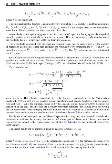
28 <strong>qreg</strong> — Quantile regression<br />
F −1<br />
Y<br />
(τ) ≈ F −1<br />
−1<br />
Y<br />
(τ + h) − FY (τ − h)<br />
dt<br />
2h<br />
where h is the bandwidth.<br />
= ξ τ+h − ξ τ−h<br />
2h<br />
= ŝ τ (4)<br />
The empirical quantile function is computed by first estimating β τ+h and β τ−h , and then computing<br />
̂F −1<br />
Y<br />
(τ + h) = x′̂βτ+h −1<br />
and ̂F<br />
Y<br />
(τ − h) = x′̂βτ−h , where x is the sample mean of the independent<br />
variables x. These quantities are then substituted into (4).<br />
Alternatively, as the option suggests, vce(iid, residual) specifies that <strong>qreg</strong> use the empirical<br />
quantile function of the residuals to estimate the sparsity. Here we substitute F ɛ , the distribution of<br />
the residuals, for F Y , which only differ by their first moments.<br />
The k residuals associated with the linear programming basis will be zero, where k is the number<br />
of regression coefficients. These zero residuals are removed before computing the τ + h and τ − h<br />
−1<br />
−1<br />
−1<br />
quantiles, ε (τ+h) = ̂F ɛ (τ + h) and ε (τ−h) = ̂F ɛ (τ − h). The ̂F ɛ estimates are then substituted<br />
for F −1<br />
Y<br />
in (4).<br />
Each of the estimators for the sparsity function depends on a bandwidth. The vce() suboption bwidth<br />
specifies the bandwidth method to use. The three bandwidth options and their citations are hsheather<br />
(Hall and Sheather 1988), bofinger (Bofinger 1975), and chamberlain (Chamberlain 1994).<br />
Their formulas are<br />
h s = n −1/3 Φ −1 ( 1 − α 2<br />
h b = n −1/5 [ 9<br />
2 φ{2Φ−1 (τ)} 4<br />
{2Φ −1 (τ) 2 + 1} 2 ]1/5<br />
h c = Φ −1 ( 1 − α 2<br />
) 2/3<br />
[ 3<br />
2 × φ{Φ−1 (τ)} 4<br />
) √ τ(1 − τ)<br />
n<br />
2Φ −1 (τ) 2 + 1<br />
where h s is the Hall–Sheather bandwidth, h b is the Bofinger bandwidth, h c is the Chamberlain<br />
bandwidth, Φ() and φ() are the standard normal distribution and density functions, n is the sample<br />
size, and 100(1 − α) is the confidence level set by the level() option. Koenker (2005) discusses the<br />
derivation of the Hall–Sheather and the Bofinger bandwidth formulas. You should avoid modifying<br />
the confidence level when replaying estimates that use the Hall–Sheather or Chamberlain bandwidths<br />
because these methods use the confidence level to estimate the coefficient standard errors.<br />
Finally, the vce() suboption kernel(kernel) specifies that <strong>qreg</strong> use one of several kernel-density<br />
estimators to estimate the sparsity function. kernel allows you to choose which kernel function to<br />
use, where the default is the Epanechnikov kernel. See [R] kdensity for the functional form of the<br />
eight kernels.<br />
] 1/3<br />
The kernel bandwidth is computed using an adaptive estimate of scale<br />
(<br />
r<br />
)<br />
q<br />
h k = min ̂σ, × { Φ −1 (τ + h) − Φ −1 (τ − h) }<br />
1.34<br />
where h is one of h s , h b , or h c ; r q is the interquartile range; and ̂σ is the standard deviation of y;<br />
see Silverman (1992, 47) and Koenker (2005, 81) for discussions. Let ̂fɛ (ε i ) be the kernel density<br />
estimate for the ith residual, and then the kernel estimator for the sparsity function is<br />
ŝ τ =<br />
nh k<br />
∑ n<br />
i=1 ̂f ɛ (ε i )


