

qreg - Stata
qreg - Stata
qreg - Stata

You also want an ePaper? Increase the reach of your titles
YUMPU automatically turns print PDFs into web optimized ePapers that Google loves.
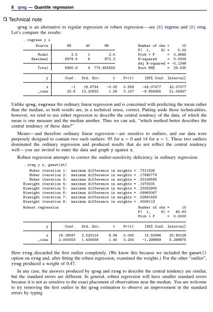
8 <strong>qreg</strong> — Quantile regression<br />
Technical note<br />
<strong>qreg</strong> is an alternative to regular regression or robust regression—see [R] regress and [R] rreg.<br />
Let’s compare the results:<br />
. regress y x<br />
Source SS df MS Number of obs = 10<br />
F( 1, 8) = 0.00<br />
Model 2.5 1 2.5 Prob > F = 0.9586<br />
Residual 6978.4 8 872.3 R-squared = 0.0004<br />
Adj R-squared = -0.1246<br />
Total 6980.9 9 775.655556 Root MSE = 29.535<br />
y Coef. Std. Err. t P>|t| [95% Conf. Interval]<br />
x -1 18.6794 -0.05 0.959 -44.07477 42.07477<br />
_cons 20.6 13.20833 1.56 0.157 -9.858465 51.05847<br />
Unlike <strong>qreg</strong>, regress fits ordinary linear regression and is concerned with predicting the mean rather<br />
than the median, so both results are, in a technical sense, correct. Putting aside those technicalities,<br />
however, we tend to use either regression to describe the central tendency of the data, of which the<br />
mean is one measure and the median another. Thus we can ask, “which method better describes the<br />
central tendency of these data?”<br />
Means—and therefore ordinary linear regression—are sensitive to outliers, and our data were<br />
purposely designed to contain two such outliers: 95 for x = 0 and 14 for x = 1. These two outliers<br />
dominated the ordinary regression and produced results that do not reflect the central tendency<br />
well—you are invited to enter the data and graph y against x.<br />
Robust regression attempts to correct the outlier-sensitivity deficiency in ordinary regression:<br />
. rreg y x, genwt(wt)<br />
Huber iteration 1: maximum difference in weights = .7311828<br />
Huber iteration 2: maximum difference in weights = .17695779<br />
Huber iteration 3: maximum difference in weights = .03149585<br />
Biweight iteration 4: maximum difference in weights = .1979335<br />
Biweight iteration 5: maximum difference in weights = .23332905<br />
Biweight iteration 6: maximum difference in weights = .09960067<br />
Biweight iteration 7: maximum difference in weights = .02691458<br />
Biweight iteration 8: maximum difference in weights = .0009113<br />
Robust regression Number of obs = 10<br />
F( 1, 8) = 80.63<br />
Prob > F = 0.0000<br />
y Coef. Std. Err. t P>|t| [95% Conf. Interval]<br />
x 18.16597 2.023114 8.98 0.000 13.50066 22.83128<br />
_cons 2.000003 1.430558 1.40 0.200 -1.298869 5.298875<br />
Here rreg discarded the first outlier completely. (We know this because we included the genwt()<br />
option on rreg and, after fitting the robust regression, examined the weights.) For the other “outlier”,<br />
rreg produced a weight of 0.47.<br />
In any case, the answers produced by <strong>qreg</strong> and rreg to describe the central tendency are similar,<br />
but the standard errors are different. In general, robust regression will have smaller standard errors<br />
because it is not as sensitive to the exact placement of observations near the median. You are welcome<br />
to try removing the first outlier in the <strong>qreg</strong> estimation to observe an improvement in the standard<br />
errors by typing


