2000 Tomei - Robust adaptive friction compensation for tracking control of robot manipulators.pdf
2000 Tomei - Robust adaptive friction compensation for tracking control of robot manipulators.pdf
2000 Tomei - Robust adaptive friction compensation for tracking control of robot manipulators.pdf

You also want an ePaper? Increase the reach of your titles
YUMPU automatically turns print PDFs into web optimized ePapers that Google loves.
2164 IEEE TRANSACTIONS ON AUTOMATIC CONTROL, VOL. 45, NO. 6, JUNE <strong>2000</strong><br />
where a = 8 T (1)K 01<br />
e 8(1)k p and b = 8 T (1)K 01<br />
e 8 0 (1)k p. Note<br />
that a> 0. Substituting (41) into (42) and after some manipulation,<br />
we obtain<br />
"(1) = a<br />
2b<br />
sin 1 0<br />
2+a 2+a 1 2: (43)<br />
The bending angle can also be calculated from the flexible coordinate p<br />
(1) = (8 0 (1)) T p = b(s 1x 2 0 c 1x 2 ) 0 c1 2 (44)<br />
where c =(8 0 (1)) T K 01<br />
e 8 0 (1)k p . Substituting (41) into (44) yields<br />
(1) = 00:5b sin 1 0 0:5b"(1) 0 c1 2: (45)<br />
From (43) and (45), it is simple to derive<br />
(1) = 0<br />
b<br />
2+a<br />
sin 1 0<br />
2c + ac 0 b2<br />
2+a<br />
1 2: (46)<br />
Note that ac 0 b 2 0. By substituting (25) into (46), we obtain<br />
b<br />
(1) = 0<br />
2+a + sin 1 0 <br />
1 (47)<br />
2+a + <br />
where =2c + ac 0 b 2 . Clearly, is positive. Substituting (47) into<br />
(43) derives<br />
"(1) =<br />
a + ac 0 b2<br />
2+a + sin 1 0 2b<br />
1: (48)<br />
2+a + <br />
Substituting (47) and (48) into (40) yields a constraint equation only<br />
on 1:<br />
4+2a + 0 b cos 1 2+a + 0 2b<br />
1 + sin 1<br />
2+a + <br />
2(2 + a + )<br />
a + ac<br />
0<br />
0 b2<br />
sin 21 =0: (49)<br />
4(2 + a + )<br />
It can be proved that this equation has such a unique solution: 1 =0<br />
[12]. There<strong>for</strong>e, we conclude that (1) = 0 from (47) and "(1) =<br />
0 from (48), which implies that both 1 1 and 1 2 are zero. From<br />
(36) and (37), we conclude that the position errors 1x 1 ; 1x 1 ) and<br />
(1x 2 ; 1x 2 ) are zero.<br />
REFERENCES<br />
[1] A. Bloch, M. Reyhanoglu, and N. H. McClamroch, “Control and stabilization<br />
<strong>of</strong> nonholonomic dynamic systems,” IEEE Trans. Automat.<br />
Contr., vol. 37, pp. 1756–1757, 1992.<br />
[2] R. W. Brockett et al., “Asymptotic stability and feedback stabilization,”<br />
in Differential Geometric Control Theory, S. B. W. Brockett et al.,<br />
Eds. Boston: Birkhauser, 1983, pp. 181–191.<br />
[3] T. Fukuda, “Flexibility <strong>control</strong> <strong>of</strong> elastic <strong>robot</strong>ic arm,” J. Rob. Syst., vol.<br />
2, no. 1, pp. 73–88, 1985.<br />
[4] Z. H. Luo, “Direct strain feedback <strong>control</strong> <strong>of</strong> flexible <strong>robot</strong> arms: New<br />
theoretical and experimental results,” IEEE Trans. Automat. Contr., vol.<br />
38, pp. 1610–1622, Nov. 1993.<br />
[5] Y. H. Liu and S. Arimoto, “Distributively <strong>control</strong>ling two <strong>robot</strong>s handling<br />
an object in the task space without and communication,” IEEE<br />
Trans. Automat. Contr., vol. 41, pp. 1193–1198, Aug. 1996.<br />
[6] K. Kosuge, M. Sakai, and K. Kanitani, “Manipulation <strong>of</strong> a flexible object<br />
by dual <strong>manipulators</strong>,” in Proc. IEEE Int. Conf. Robot. and Automat.,<br />
1995, pp. 318–323.<br />
[7] W. Kraus Jr. and B. J. MaCarragher, “Force fields in the manipulation <strong>of</strong><br />
flexible materials,” in Proc. IEEE Int. Conf. Robot. Automat., 1996, pp.<br />
2352–2357.<br />
[8] J. K. Mills, “Multi-manipulator <strong>control</strong> <strong>for</strong> fixtureless assembly <strong>of</strong> elastically<br />
de<strong>for</strong>mable parts,” in Proc. Japan-USA Symp. Flexible Automat.,<br />
1992, pp. 1565–1572.<br />
[9] H. Nakagaki, K. Kitagaki, and H. Tsukune, “Study <strong>of</strong> intersection task<br />
<strong>of</strong> a flexible beam into a hole,” in Proc. IEEE Int. Conf. Robot. Automat.,<br />
1995, pp. 330–335.<br />
[10] G. Oriolo and Y. Nakamura, “Control <strong>of</strong> mechanical systems with<br />
second-order nonholonomic constraints: Underactuated <strong>manipulators</strong>,”<br />
in Proc. IEEE CDC, 1991, pp. 2398–2403.<br />
[11] W. Nguyen and J. K. Mills, “Multi-<strong>robot</strong> <strong>control</strong> <strong>for</strong> flexible fixtureless<br />
assembly <strong>of</strong> flexible sheet metal auto body parts,” in Proc. IEEE Int.<br />
Conf. Robot. Automat., 1996, pp. 2340–2345.<br />
[12] D. Sun, “Cooperative <strong>control</strong> <strong>of</strong> two-manipulator systems handling flexible<br />
objects,” Ph.D. dissertation, The Chinese Univ. Hong Kong, Shatin,<br />
Hong Kong, 1997.<br />
[13] D. Sun, Y. H. Liu, and J. K. Mills, “Cooperative <strong>control</strong> <strong>of</strong> a two-manipulator<br />
system handling a general flexible object,” in Proc. IEEE/RSJ<br />
Conf. Intell. Robots Syst., 1997, pp. 5–10.<br />
[14] T. J. Tarn et al., “Design if dynamic <strong>control</strong> <strong>of</strong> two cooperating <strong>robot</strong><br />
arms closed chain <strong>for</strong>mulation,” in Proc. IEEE Int. Conf. Robot Automat.,<br />
Raleigh, 1987, pp. 7–13.<br />
[15] I. D. Walker, R. A. Freeman, and S. I. Marcus, “Analysis <strong>of</strong> motion and<br />
internal loading <strong>of</strong> objects grasped by multiple cooperating <strong>manipulators</strong>,”<br />
Int. J. Robot. Res., vol. 10, no. 4, pp. 396–409, 1989.<br />
[16] J. T. Wen and K. Kreutz-Delgado, “Motion and <strong>for</strong>ce <strong>for</strong> multiple <strong>robot</strong>ic<br />
<strong>manipulators</strong>,” Automatica, vol. 28, no. 4, pp. 729–743, 1992.<br />
[17] T. Yukawa et al., “Stability <strong>of</strong> <strong>control</strong> system in handling <strong>of</strong> a flexible<br />
object by rigid arm <strong>robot</strong>s,” in Proc. IEEE Int. Conf. Robot. Automat.,<br />
1996, pp. 2332–2339.<br />
[18] Y. F. Zheng and M. Z. Chen, “Trajectory planning <strong>for</strong> two <strong>manipulators</strong><br />
to de<strong>for</strong>m flexible objects,” in Proc. IEEE Int. Conf. Robot. Automat.,<br />
1993, pp. 1019–1024.<br />
[19] Y. F. Zheng, R. Pei, and C. Chen, “Strategies <strong>for</strong> automatic assembly<br />
<strong>of</strong> de<strong>for</strong>mable objects,” in IEEE Int. Conf. Robot. Automat., 1991, pp.<br />
2708–2715.<br />
[20] K. Y. Wichlund, O. J. Sørdalen, and O. Egeland, “Control <strong>of</strong> vehicles<br />
with second-order nonholonomic constraints: Underactuated vehicles,”<br />
in Proc. Eur. Contr. Conf., 1995, pp. 3086–3091.<br />
<strong>Robust</strong> Adaptive Friction Compensation <strong>for</strong> Tracking<br />
Control <strong>of</strong> Robot Manipulators<br />
Patrizio <strong>Tomei</strong><br />
Abstract—The <strong>tracking</strong> problem is considered <strong>for</strong> <strong>robot</strong> <strong>manipulators</strong><br />
with unknown parameters and dynamic <strong>friction</strong>, in the presence<br />
<strong>of</strong> bounded disturbances and/or modeling uncertainties. The authors<br />
design a robust <strong>adaptive</strong> <strong>control</strong> algorithm which guarantees arbitrary<br />
disturbance attenuation. If the disturbances belong to , asymptotic<br />
<strong>tracking</strong> is also achieved.<br />
Index Terms—Disturbance attenuation, dynamic <strong>friction</strong>, <strong>robot</strong>ic <strong>manipulators</strong>,<br />
robust <strong>adaptive</strong> <strong>control</strong>.<br />
I. INTRODUCTION<br />
High-per<strong>for</strong>mance position <strong>tracking</strong> <strong>control</strong> <strong>of</strong> mechanical systems<br />
cannot be per<strong>for</strong>med adequately if <strong>friction</strong> phenomena are not properly<br />
taken into account. Moreover, a more accurate representation <strong>of</strong> <strong>friction</strong><br />
should allow the <strong>control</strong> gains (and there<strong>for</strong>e the feedback <strong>control</strong><br />
component) to be decreased, since the <strong>friction</strong> disturbance terms<br />
could be compensated by the feed<strong>for</strong>ward component <strong>of</strong> the <strong>control</strong><br />
algorithm. The previous statement understands that <strong>friction</strong> is exactly<br />
known, and this, in turn, implies that the <strong>friction</strong> parameters are known<br />
Manuscript received November 1, 1999. Recommended by Associate Editor,<br />
G. Tao. This work was supported in part by MURST and in part by ASI.<br />
The author is with the Dipartimento di Ingegneria Elettronica, Università di<br />
Roma ‘Tor Vergata’ 00133 Roma, Italy.<br />
Publisher Item Identifier S 0018-9286(00)04217-3.<br />
0018–9286/00$10.00 © <strong>2000</strong> IEEE
IEEE TRANSACTIONS ON AUTOMATIC CONTROL, VOL. 45, NO. 6, JUNE <strong>2000</strong> 2165<br />
and the <strong>friction</strong> state variables are available from measurements. Un<strong>for</strong>tunately,<br />
this is rarely the case, so that <strong>adaptive</strong> (or robust) techniques<br />
are needed to deal with uncertain parameters and state observers are<br />
needed to estimate the <strong>friction</strong> unmeasured variables.<br />
For the <strong>tracking</strong> <strong>control</strong> <strong>of</strong> <strong>robot</strong> <strong>manipulators</strong>, other parameter uncertainties<br />
related to the mechanical structure have to be taken into account.<br />
By considering only linear viscous <strong>friction</strong> effects, many <strong>adaptive</strong><br />
<strong>control</strong>s <strong>for</strong> <strong>robot</strong> <strong>manipulators</strong> have been proposed in the literature<br />
(see [1]–[3] <strong>for</strong> a survey). Since time-varying disturbances are not<br />
considered in all <strong>of</strong> these schemes, they may not work satisfactorly in<br />
the presence <strong>of</strong> disturbance torques and/or modeling uncertainties. On<br />
the other hand, the robust and the H1 <strong>control</strong>lers developed in [4]–[7]<br />
allow <strong>for</strong> unstructured time-varying disturbances but they are unable to<br />
guarantee asymptotic <strong>tracking</strong> (even though the disturbances vanish).<br />
Moreover, disturbance attenuation is achieved by en<strong>for</strong>cing the feedback<br />
<strong>control</strong> component to counteract the perturbations due to exogeneous<br />
disturbances and modeling uncertainties. To retain both the<br />
advantages <strong>of</strong> robust and <strong>adaptive</strong> <strong>control</strong>s, in [8] a robust <strong>adaptive</strong><br />
<strong>control</strong>ler was designed which tolerates time-varying parameters and<br />
disturbances, and guarantees asymptotic <strong>tracking</strong> when parameters are<br />
constant and disturbances are vanishing. However, the transient per<strong>for</strong>mance<br />
depends upon disturbance bounds and cannot be arbitrarily<br />
improved. An <strong>adaptive</strong> <strong>control</strong> <strong>for</strong> mechanical systems with nonlinear<br />
<strong>friction</strong> was proposed in [9], while in [10] the <strong>friction</strong> was treated as a<br />
nonlinearly parametrized function. In both papers time-varying disturbances<br />
are not allowed and transient per<strong>for</strong>mance are not guaranteed.<br />
A robust <strong>adaptive</strong> <strong>control</strong>ler with transient per<strong>for</strong>mance and arbitrary<br />
disturbance attenuation has been proposed in [11], where only instantaneous<br />
<strong>friction</strong> is taken into account, without modeling dynamical effects.<br />
As far as dynamically modeled <strong>friction</strong> is concerned, the problem<br />
<strong>of</strong> its <strong>compensation</strong> in a DC motor along with a new dynamic model<br />
was treated in [12], assuming that all parameters were known. A further<br />
extension <strong>of</strong> this result to the case in which the <strong>friction</strong> <strong>for</strong>ce depends<br />
linearly on only one unknown parameter was given in [13] <strong>for</strong> the<br />
stabilization problem. A discontinuous <strong>tracking</strong> <strong>control</strong> law has been<br />
recently proposed in [14] <strong>for</strong> <strong>adaptive</strong> <strong>friction</strong> <strong>compensation</strong> in <strong>robot</strong><br />
<strong>manipulators</strong>, where more uncertainty is allowed in the <strong>friction</strong> terms.<br />
However, none <strong>of</strong> the previous works takes into account the action <strong>of</strong><br />
bounded time-varying disturbances (with unknown bound), due to exogeneous<br />
disturbance <strong>for</strong>ces or to bounded modeling uncertainty, as well<br />
as transient per<strong>for</strong>mance bounds which are considered in this paper.<br />
We present a robust <strong>adaptive</strong> <strong>tracking</strong> <strong>control</strong>ler which guarantees<br />
arbitrary attenuation on the joint position and joint velocity <strong>tracking</strong><br />
errors <strong>of</strong> the effects <strong>of</strong> bounded disturbances. The proposed <strong>control</strong>ler<br />
achieves asymptotic <strong>tracking</strong> when disturbances belong to L2. Dynamic<br />
<strong>friction</strong> <strong>for</strong>ces depending on unknown parameters are taken into<br />
account, which are not available from measurements.<br />
II. MAIN RESULT<br />
We consider a <strong>robot</strong> manipulator consisting <strong>of</strong> n +1links interconnected<br />
by n joints whose dynamic model is<br />
B(q; )q + C(q; _q; )_q + h(q; ) +F0z<br />
+ F1 _z + F2 _q = u + d(t)<br />
j _q j j<br />
_z j = 0f0j zj +_qj; 1 j n (1)<br />
g j (_q j )<br />
in which the vector q = [q1; 111;q n ] T represents the joint relative<br />
displacements, the vector z = [z1; 111;z n ] T takes into account the<br />
<strong>friction</strong> dynamics (see [12]), the vector 2 R m is the vector <strong>of</strong> the<br />
kinematic and dynamic parameters <strong>of</strong> <strong>robot</strong> and actuators which enters<br />
linearly in the <strong>robot</strong> equations, the vector u denotes generalized <strong>for</strong>ces<br />
(<strong>for</strong>ces or torque) applied at the joints, B(q; ) is the symmetric positive<br />
definite inertia matrix, and C(q; _q; )_q represents Coriolis and<br />
centripetal <strong>for</strong>ces. The vector z represents the average deflection between<br />
the contact surfaces during the stiction phase. The <strong>friction</strong> <strong>for</strong>ce<br />
F = F0z + F1 _z + F2 _q consists <strong>of</strong> three terms: the viscous <strong>friction</strong><br />
F2 _q, the stiffness <strong>for</strong>ce F0z, and the damping <strong>for</strong>ce F1 _z, with F i diagonal<br />
positive semidefinite matrices (F i =diag[f ij ]). The disturbance<br />
<strong>for</strong>ces due to exogeneous disturbances are grouped into the vector d(t),<br />
which is assumed to be bounded; d(t) may also contain bounded unstructured<br />
modeling uncertainties. The vector is assumed to be unknown<br />
and to belong to a known compact set, which <strong>for</strong> the sake <strong>of</strong><br />
simplicity is supposed to be a closed ball centered at N (the nominal<br />
value <strong>of</strong> ). As stated in [12], by measuring the steady-state <strong>friction</strong><br />
<strong>for</strong>ce when the velocity _q is constant, the functions g j and the matrix<br />
F0 can be determined and, there<strong>for</strong>e, they are supposed to be known.<br />
The case in which they are not known will be addressed in Remark 2.4.<br />
The functions g j are always positive and decrease monotonically from<br />
g j (0) as _q j increases. As shown in [12], the z j variables are always<br />
bounded and, in particular, if jz j(0)j g j(0) then jz j(t)j g j(0),<br />
<strong>for</strong> any t 0. The matrices F1 and F2 are supposed to be unknown<br />
and to belong to a known compact set; the nominal values are denoted<br />
by F1N and F2N . The choice <strong>of</strong> C(q; _q; ) is not unique; we choose<br />
the elements <strong>of</strong> C as follows [1], [15]:<br />
C ij = 1 2<br />
_q T @B ij<br />
@q + n<br />
k=1<br />
@B ik<br />
@q j<br />
0 @B jk<br />
q i<br />
_q k (2)<br />
where i; j = 1; 111;n, so that the matrix _ B(q; ) 0 2C(q; _q; ) is<br />
skew-symmetric. We assume that only the position q(t) and the velocity<br />
_q(t) are available from measurements. For the <strong>robot</strong> model (1),<br />
we consider the <strong>adaptive</strong> <strong>tracking</strong> problem <strong>for</strong>mulated in the following<br />
definition.<br />
Definition 2.1: The robust <strong>adaptive</strong> <strong>tracking</strong> problem with arbitrary<br />
disturbance attenuation is said to be globally solvable <strong>for</strong><br />
the <strong>robot</strong> manipulator (1) if, given any smooth bounded reference<br />
trajectory q r (t) with bounded derivatives _q r (t) and q r (t), a parametrized<br />
<strong>adaptive</strong> <strong>control</strong> law (k > 0)u = u(q; _q; q r; _q r; q r; ^; k);<br />
_^ = (q; _q; q r ; _q r ; q r ; ^; k), exists such that <strong>for</strong> the closed-loop<br />
system: i) (boundedness) k^(t)k; kq(t)k, and k _q(t)k are bounded<br />
8t 0; ii) (arbitrary disturbance attenuation) the following inequality<br />
holds 8t >t0 and 8t0 0:<br />
2<br />
t<br />
q( ) 0 q r( )<br />
d<br />
t<br />
_q( ) 0 _q r( )<br />
2(t0)+ 1 t<br />
k 1(M )(t 0 t0) + kd( )k 2 d (3)<br />
t<br />
where 2 is a nonnegative constant depending on initial conditions<br />
q(t0)0q r (t0); _q(t0)0 _q r (t0);z(t0); ^(t0) and 1 is a positive constant<br />
depending only on a known constant M ; and iii) (asymptotic <strong>tracking</strong>)<br />
if d(t) 2 L2 \ L1, then<br />
lim<br />
t!1 q(t) 0 q r(t)<br />
_q(t) 0 _q r(t)<br />
=0:<br />
The following result shows how an <strong>adaptive</strong> <strong>tracking</strong> <strong>control</strong> which<br />
solves the problem given in the previous definition may be actually<br />
designed.<br />
Theorem 2.1: The robust <strong>adaptive</strong> <strong>tracking</strong> problem with arbitrary<br />
disturbance attenuation is globally solvable <strong>for</strong> the <strong>robot</strong> system (1).
2166 IEEE TRANSACTIONS ON AUTOMATIC CONTROL, VOL. 45, NO. 6, JUNE <strong>2000</strong><br />
Pro<strong>of</strong>: Let x 1 = q; x 2 = _q, so that (1) is written as<br />
_x 1 = x 2<br />
B(x 1;)_x 2 = 0C(x 1;x 2;)x 2 0 h(x 1;) 0 F 0z<br />
0 (F 1 + F 2)x 2 + F 18(x 2)z + u + d(t)<br />
_z = 08(x 2 )z + x 2 (4)<br />
where 8(x 2 )=diag[f 0j (jx 2j j)=(g j (x 2j ))] = 4 diag[ j (x 2j )]. Per<strong>for</strong>m<br />
the change <strong>of</strong> coordinates ~x 1 = x 1 0 q r; ~x 2 = x 2 0 x 3 2 with<br />
x 3 2 = 0K 1 (x 1 0 q r )+ _q r and K 1 a symmetric positive definite matrix<br />
(K 1 > 0). Let 0 a (m + n) 2 n matrix such that 0C(x 1 ;x 2 ;)<br />
(0K 1~x 1 +_q r)0h(x 1;)0(F 1 +F 2) x 2 +B(x 1;)K 1 (x 2 0 _q r)0<br />
B(x 1 ;)q r = 0 T (x 1 ;x 2 ;q r ; _q r ; q r ) in which = [ T ;f 11 +<br />
f 21 ; 111;f 1n + f 2n ] T 4 = N + a with f ij the jth diagonal element <strong>of</strong><br />
matrix F i . Let aM be the (known) largest value <strong>of</strong> k a k. We obtain<br />
_~x 1 = 0K 1 ~x 1 +~x 2<br />
B(x 1 ;) _~x 2 + C(x 1 ;x 2 ;)~x 2 = 0F 0 z + F 1 8(x 2 )z<br />
+0 T (x 1 ;x 2 ;q r ; _q r ; q r ) + d(t)+u<br />
_z = 08(x 2)z + x 2: (5)<br />
Since we know a bound <strong>for</strong> the z-variables kz(t)k k[g 1 (0); 111;<br />
g n (0)]k = 4 z M ; 8t 0, we define (k >0;K 2 > 0)<br />
u = 00 T ( N + ^ a )+F 0 ^z 0 (F 1N + 1F ^ 1 )8^z<br />
0 k 4 ~x2 0 k 4 0T 0~x 2 0 K 2~x 2 0 ~x 1 + v(t) (6)<br />
with (k^z(0)k z M)<br />
_^z =Proj(08^z + x 2 0 F 0 ~x 2 + F 1N 8~x 2 ; ^z) (7)<br />
where the dynamics <strong>of</strong> the estimates ^ a and 1F ^ 1 and the <strong>control</strong> v(t)<br />
are yet to be defined, while Proj(y; ^) is the smooth projection algorithm<br />
introduced in [16], which in this case is given by: Proj(y; ^) =y,<br />
if p(^) 0; Proj(y; ^) =y, ifp(^) 0 and p^(^)y 0;,<br />
Proj(y; ^) =[I 0 (p(^)p^(^) T p^(^))=(kp^(^)k 2 )]y; if p(^) > 0<br />
with<br />
and p^(^)y >0;<br />
p(^) =(^ T ^ 0 <br />
2<br />
M)=( 2 +2 M );p^(^) =(dp(^))=(d^)<br />
and an arbitrary positive real. The projection algorithm<br />
is such that, if<br />
_^ = Proj(y; ^) and k^(0)k M then:<br />
k^(t)k M + ; 8t 0; Proj(y; ^) is Lipschitz and continuous;<br />
kProj(y; ^)k kyk; ~ T Proj(y; ^) ~ T y. From (5) and (6),<br />
we obtain ( ~ = 0 ^)<br />
_~x 1 = 0K 1~x 1 +~x 2<br />
B _~x 2 + C ~x 2 =0 T ~ a 0 ~x 1 0 k 4 0 k 4 0T 0 0 K 2 ~x 2<br />
0 [F 0 + F 1N 8+1F 18]~z + 8 T (x 2; ^z) ~ b + d + v<br />
(8)<br />
where b = [1f 11 ; 111; 1f 1n ] T and 8 T (x 2 ; ^z) ~ b = (1F 1 0<br />
1F ^ 1 )8(x 2 )^z. Let bM be the largest (known) value <strong>of</strong> k b k. Consider<br />
the function<br />
W = 1 2 ~xT 1 ~x 1 +~x T 2 B(x 1;)~x 2 +~z T ~z : (9)<br />
Its time derivative, in view <strong>of</strong> (8), is such that<br />
_W = 0~x T 1 K 1 ~x 1 +~x T 1 ~x 2 + 1 2 _ ~xT 2 B~x 2 +~x T 2 0C ~x 2 +0 T a<br />
~<br />
0 ~x 1 0 k 4 ~x 2 0 k 4 0T 0~x 2 0 K 2 ~x 2 0 F 0 ~z + F 1N 8~z<br />
+1F 1 8~z + 8 T ~ b + d + v +~z T (08z + x 2 0 _^z) (10)<br />
which, recalling property d) <strong>of</strong> Proj and the skew-symmetry <strong>of</strong> _ B02C,<br />
implies<br />
_W 0~x T 1 K 1~x 1 0 ~x T 2 K 2~x 2 + kdk2<br />
+ 1 <br />
k k ~ T ~ a a<br />
+~x T 2 [8 T b<br />
~ + v(t)] + ~x T 2 1F 18~z 0 ~z T 8~z: (11)<br />
Since ~x T 2 1F 1 8~z 0 ~z T n<br />
8~z = [~x j=1 2j ~z j j 1f 1j 0~z 2 j j ] =<br />
n<br />
j=1 j (~x 2j ~z j 1f 1j 0~z 2 j )= n j=1 j[0((1=2)~x 2j 1f 1j 0 ~z j ) 2<br />
+(1=4)~x 2 2j1f1j] 2 from (11), we obtain<br />
Now, choose<br />
_W 0~x T 1 K 1~x 1 0 ~x T 2 K 2~x 2 + kdk2<br />
k<br />
+~x T 2 [8 T ~ b + v(t)] + 1 4<br />
n<br />
j=1<br />
+ k~ a k 2<br />
k<br />
j ~x 2 2j1f 2 1j: (12)<br />
v = 0 k 4 8T (x 2; ^z)8(x 2; ^z)~x 2 0 8T (x 2 ; ~x 2 ) ^ c<br />
4<br />
0 k 16 8T (x 2 ; ~x 2 )8(x 2 ; ~x 2 )~x 2 (13)<br />
where ^ c is an estimate <strong>of</strong> c =[1f11; 2 111; 1f1n] 2 T , which belongs<br />
n<br />
to a closed ball <strong>of</strong> known radius cM . Since j=1 j ~x 2 2j1f 2 1j =<br />
~x T 2 8 T (x 2 ; ~x 2 ) c , from (12), (13) we have<br />
_W 0~x T 1 K 1 ~x 1 0 ~x T 2 K 2 ~x 2 + kdk2<br />
k<br />
+ 1 k k~ a k 2 + k ~ b k 2 + k ~ c k 2 : (14)<br />
For the dynamics <strong>of</strong> the estimates we use a gradient algorithm with<br />
projection as given in the following:<br />
_^ a = Proj(0(x 1 ;x 2 ;q r ; _q r ; q r )~x 2 ; ^ a ); k^ a (0)k aM<br />
_^ b = Proj(8(x 2 ; ^z)~x 2 ; ^ b ); k^ b (0)k bM<br />
_^ c = Proj(8(x 2 ; ~x 2 )~x 2 ; ^ c ); k^ c (0)k cM : (15)<br />
The projections guarantee the boundedness <strong>of</strong> ^z; ^ a; ^ b ; ^ c and, consequently<br />
(since z(t) is bounded), <strong>of</strong> ~z; ~ a ; ~ b ; ~ c . By virtue <strong>of</strong> (9) and<br />
(14) it follows that ~x 1 and ~x 2 are bounded so that property i) <strong>of</strong> Definition<br />
2.1 is proved. Integrating (14), we obtain<br />
t<br />
t<br />
~x T 1 K 1 ~x 1 +~x T 2 K 2 ~x 2 d<br />
t<br />
W (t 0 )+ 1 kdk 2 d<br />
k<br />
t<br />
+ 1 k sup (k ~ a k 2 + k ~ b k 2 + k ~ c k 2 )(t 0 t 0 ): (16)<br />
2[t ;t]<br />
By virtue <strong>of</strong> property a) <strong>of</strong> the operator Proj, we have, 8t <br />
0; k^ a (t)k aM + ; k^ b (t)k bM + ; k^ c (t)k cM + <br />
so that, with a proper redefinition <strong>of</strong> k, (3) in Definition 2.1 easily<br />
follows. As far as property iii) is concerned, consider the function<br />
V = W + 1 2 ~ T a ~ a + ~ T b ~ b + ~ T c ~ c (17)<br />
whose time derivative, taking (10), (13), (15) and property d) <strong>of</strong> Proj<br />
into account, is such that<br />
_V 0~x T 1 K 1 ~x 1 0 ~x T 2 K 2 ~x 2 + 1 k kd(t)k2 : (18)<br />
From (18), since d(t) 2 L 2 , we obtain lim t!1 t 0 (~xT 1 K 1 ~x 1 +<br />
~x T 2 K 2 ~x 2 ) d < 1. Since by (5), _~x 1 and _~x 2 are bounded, by the<br />
Barbalat lemma (see [17]), property iii) in Definition 2.1 follows.<br />
Remark 2.1: By virtue <strong>of</strong> the disturbance attenuation terms in (6)<br />
and (13), the adaptation dynamics <strong>for</strong> ^ a; ^ b , and ^ c may be switched
IEEE TRANSACTIONS ON AUTOMATIC CONTROL, VOL. 45, NO. 6, JUNE <strong>2000</strong> 2167<br />
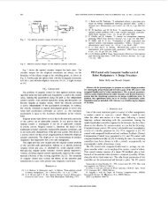
Fig. 1.<br />
Tracking and observer error, reference, and torque.<br />
<strong>of</strong>f at any time without compromising the stability <strong>of</strong> the closed loop<br />
system, as apparent from (9) and (14), and preserving properties i) and<br />
ii) in Definition 2.1.<br />
Remark 2.2: If, in addition to the L 2 bound represented by the inequality<br />
(3) in Definition II.1, an L1 bound <strong>of</strong> this kind is required<br />
q(t) 0 q r (t)<br />
_q(t) 0 _q r<br />
4(t 0)+ p 1 3( M )<br />
(t) k<br />
+ p 1<br />
sup kd( )k; 8t<br />
k<br />
t 0<br />
2[t ;t]<br />
K 1 and K 2 should be chosen as: K 1 = kK 1 ;K 2 = kK 2 with K 1 ><br />
0; K 2 > 0.<br />
Remark 2.3: The proposed robust <strong>adaptive</strong> <strong>control</strong> may be easily<br />
modified to deal with time-varying parameters, following the design<br />
given in [11].<br />
Remark 2.4: The only parameters which are a priori assumed to be<br />
known are the entries f oj <strong>of</strong> matrix F 0 . Suppose that the actual value<br />
<strong>of</strong> F 0 (denoted by F 3 0<br />
) is different than its nominal value F 0. We can<br />
write (1) as<br />
B q + C _q + h + F 0z + F 1 _z + F 2 _q = u + d(t)<br />
_z j = 0f 0j<br />
_z 3 j = 0f 3 0j<br />
k _q j k<br />
g j (_q z j + _q j ; 1<br />
j<br />
j n (19)<br />
)<br />
k _q j k<br />
g j (_q j ) z3 j + _q j; 1 j n (20)<br />
where d(t) =d(t)+F 0 z0F 3 0<br />
z 3 . Since F 0 z0F 3 0<br />
z 3 is a time-varying<br />
bounded vector, we can treat d(t) as a time-varying bounded disturbance<br />
(even though it is state-dependent), so that (19) is still in the<br />
<strong>for</strong>m (1), with d(t) in place <strong>of</strong> d(t). Moreover, the nominal <strong>friction</strong><br />
dynamics given by the second equation in (19) contains the known coefficients<br />
f 0j, while the true <strong>friction</strong> dynamics (20) is not considered.<br />
The <strong>control</strong> law (6), (7), (13), (15) is there<strong>for</strong>e robust with respect to<br />
uncertainties on F 0. The same reasoning may be applied <strong>for</strong> uncertainties<br />
on the g j functions.<br />
III. SIMULATION RESULTS<br />
Some simulations have been carried out with reference to the current-<strong>control</strong>led<br />
DC motor illustrated in [13]: B q + f 0z + f 1<br />
_z + f 2 _q = u + d(t); _z = 0(f 0j _qj)=(a 0 + a 1e 0(_q=! )<br />
)z + _q;<br />
in which B is the total inertia (motor plus load), (f 0 z + f 1 _z + f 2 _q)<br />
is the <strong>friction</strong> torque, q is the motor shaft angular position and u is<br />
the DC motor torque. The nominal known values <strong>of</strong> parameters and<br />
disturbances are: B N =0:0025 kg/m 2 , f 0N =260Nm/rad, f 1N =<br />
0:7 Nms/rad, f 2N =0;a 0N =0:285 Nm, a 1N =0:05 Nm, ! 0N =<br />
0:01 rad/s, d N (t) = 0. Following the procedure given in Section II,<br />
we designed the <strong>control</strong> law<br />
u = 00 T ( N + ^ a )+f 0 ^z 0 (f 1N + ^ f b<br />
0j _qj<br />
) ^z 0 k ~x 2<br />
g(_q) 4<br />
0 k 4 0T 0~x 2 0 k 2 ~x 2 0 ~x 1 + v<br />
v = 0 k 4 82 ^z 2 ~x 2 0<br />
_^ a = Proj(0~x 2 ; ^ a );<br />
_^ c = Proj<br />
8~x 2 2; ^ c<br />
1 4 8^z ^ c 0 k 16 2 ~x 3 2<br />
_^z = Proj(08^z + _q 0 f 0 ~x 2 0<br />
_^ b = Proj(8^z~x 2 ; ^ b )<br />
f 1N 8~x 2 ; ^z)
2168 IEEE TRANSACTIONS ON AUTOMATIC CONTROL, VOL. 45, NO. 6, JUNE <strong>2000</strong><br />
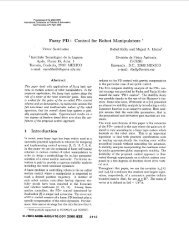
Fig. 2.<br />
Estimates <strong>of</strong> parameter deviations.<br />
with ~x 2 = _q 0 _q r + k 1(q 0 q r); g(_q) = a 0N + a 1N e 0(_q=! ) ;<br />
0 T = [k 1 (_q 0 _q r ) 0 q r ; 0 _q]; T N = [B N ;f 1N + f 2N ];<br />
8 = (f 0N j _qj)=(g(_q)). In the first set <strong>of</strong> simulations we assumed<br />
that d(t) = 0 and that the nominal values <strong>of</strong> f 0;a 0;a 1;! 0<br />
coincided with their actual values, while the actual values <strong>of</strong> the<br />
other parameters were chosen as: B = 0:0022 kg/m 2 , f 1 = 0:6<br />
Nms/rad, f 2 = 0:018 Nms/rad. The initial conditions <strong>of</strong> the motor<br />
and <strong>of</strong> the <strong>control</strong>ler were set equal to zero while the following gain<br />
constants were chosen: k = 0:1;k 1 = 5;k 2 = 25. The reference<br />
position was (as in [13]): q r (t) = 5:6 sin(0:4t) sin(0:02t). The<br />
results <strong>of</strong> the simulations are illustrated in Figs. 1 and 2, which show<br />
a satisfactory behavior <strong>of</strong> the closed-loop system. A second set <strong>of</strong><br />
simulations was then per<strong>for</strong>med with actual values <strong>of</strong> f 0 ;a 0 ;a 1 ;! 0<br />
different from their nominal values, precisely: f 0 = 280 Nm/rad,<br />
a 0 =0:3 Nm, a 1 =0:055 Nm, ! 0 =0:012 rad/s. Moreover, a torque<br />
disturbance d(t) =0:1 sin(100t) was added to perturb the system.<br />
The initial conditions and the <strong>control</strong>ler gains were left unchanged.<br />
In the corresponding results there are no appreciable differences with<br />
respect to Figs. 1 and 2, except in the input torque which has a small<br />
oscillation at the same frequency <strong>of</strong> the disturbance.<br />
IV. CONCLUSION<br />
An <strong>adaptive</strong> <strong>tracking</strong> <strong>control</strong>ler has been designed <strong>for</strong> <strong>robot</strong>s subject<br />
to dynamic <strong>friction</strong>, which is able to guarantee arbitrary disturbance<br />
attenuation on the joint position and joint velocity <strong>tracking</strong> errors <strong>of</strong><br />
the effects <strong>of</strong> modeling uncertainties and unknown bounded disturbances.<br />
The unknown parameters are supposed to belong to a known<br />
compact set while the bounds <strong>of</strong> the disturbances may be unknown.<br />
Even though the <strong>friction</strong> is dynamically modeled, only positions and<br />
velocities <strong>of</strong> the joints must be available from measurements, while<br />
the <strong>friction</strong> variables are estimated by means <strong>of</strong> a suitable observer.<br />
Three separate <strong>control</strong> components may be distinguished: disturbance<br />
attenuation terms, adaptation terms, and an observer <strong>for</strong> the <strong>friction</strong><br />
dynamics. The adaptation part is needed to guarantee asymptotic<br />
<strong>tracking</strong> <strong>for</strong> L 2 disturbances. However, the adaptation dynamics may<br />
be stopped (i.e., the parameters estimates may be frozen) without<br />
affecting the stability <strong>of</strong> the closed-loop system and still ensuring arbitrary<br />
disturbance attenuation.<br />
REFERENCES<br />
[1] J. J. Slotine and W. Li, “On the <strong>adaptive</strong> <strong>control</strong> <strong>of</strong> <strong>robot</strong> <strong>manipulators</strong>,”<br />
Int. J. Robotics Res., vol. 6, pp. 49–59, 1987.<br />
[2] P. <strong>Tomei</strong>, “Adaptive PD <strong>control</strong>ler <strong>for</strong> <strong>robot</strong> <strong>manipulators</strong>,” IEEE Trans.<br />
Robotics Automat., vol. 7, pp. 565–570, 1991.<br />
[3] R. Ortega and M. W. Spong, “Adaptive motion <strong>control</strong> <strong>of</strong> rigid <strong>robot</strong>s:<br />
A tutorial,” Automatica, vol. 25, pp. 877–888, 1989.<br />
[4] M. W. Spong, “On the robust <strong>control</strong> <strong>of</strong> <strong>robot</strong> <strong>manipulators</strong>,” IEEE<br />
Trans. Automat. Contr., vol. 37, pp. 1782–1786, 1992.<br />
[5] P. <strong>Tomei</strong>, “Tracking <strong>control</strong> <strong>of</strong> flexible joint <strong>robot</strong>s with uncertain parameters<br />
and disturbances,” IEEE Trans. Automat. Contr., vol. 39, pp.<br />
1067–1072, 1994.<br />
[6] S. Nicosia and P. <strong>Tomei</strong>, “Tracking <strong>control</strong> with disturbance attenuation<br />
<strong>for</strong> <strong>robot</strong> <strong>manipulators</strong>,” Int. J. Adapt. Contr. Sign. Proc., vol. 10, pp.<br />
443–449, 1996.<br />
[7] S. Zenieh and M. Corless, “Simple robust <strong>tracking</strong> <strong>control</strong>lers <strong>for</strong><br />
<strong>robot</strong>ic <strong>manipulators</strong>,” in Proc. 4th IFAC SYROCO, Capri, Italy, 1994,<br />
pp. 193–198.<br />
[8] G. Tao, “On robust <strong>adaptive</strong> <strong>control</strong> <strong>of</strong> <strong>robot</strong> <strong>manipulators</strong>,” Automatica,<br />
vol. 28, pp. 803–807, 1992.<br />
[9] M. Feemster, P. Vedagarbha, D. M. Dawson, and D. Haste, “Adaptive<br />
<strong>control</strong> techniques <strong>for</strong> <strong>friction</strong> <strong>compensation</strong>,” in Proc. Amer. Contr.<br />
Conf., Philadelphia, PA, 1998, pp. 1488–1492.
IEEE TRANSACTIONS ON AUTOMATIC CONTROL, VOL. 45, NO. 11, NOVEMBER <strong>2000</strong> 2169<br />
[10] A. M. Annaswamy, F. P. Skantze, and A. Loh, “Adaptive <strong>control</strong> <strong>of</strong><br />
continuous time systems with convex/concave parametrization,” Automatica,<br />
vol. 34, pp. 33–49, 1998.<br />
[11] P. <strong>Tomei</strong>, “<strong>Robust</strong> <strong>adaptive</strong> <strong>control</strong> <strong>of</strong> <strong>robot</strong>s with arbitrary transient per<strong>for</strong>mance<br />
and disturbance attenuation,” IEEE Trans. Automat. Contr.,<br />
vol. 44, pp. 654–658, 1999.<br />
[12] C. Canudas de Wit, H. Olsson, K. J. Astrom, and P. Lischinsky, “A<br />
new model <strong>for</strong> <strong>control</strong> <strong>of</strong> systems with <strong>friction</strong>,” IEEE Trans. Automat.<br />
Contr., vol. 40, pp. 419–425, 1995.<br />
[13] C. Canudas and P. Lischinsky, “Adaptive <strong>friction</strong> <strong>compensation</strong> with<br />
partially known dynamic <strong>friction</strong> model,” Int. J. Adapt. Contr. Sign.<br />
Proc., vol. 11, pp. 65–80, 1997.<br />
[14] E. Panteley, R. Ortega, and M. Gafvert, “An <strong>adaptive</strong> <strong>friction</strong> compensator<br />
<strong>for</strong> global <strong>tracking</strong> in <strong>robot</strong> <strong>manipulators</strong>,” Syst. Contr. Lett., vol.<br />
33, pp. 307–313, 1998.<br />
[15] S. Arimoto and F. Miyazaki, “Stability and robustness <strong>of</strong> PID feedback<br />
<strong>control</strong> <strong>for</strong> <strong>robot</strong> <strong>manipulators</strong> <strong>of</strong> sensory capability,” in Robotics Research,<br />
M. Brady and R. Paul, Eds. Cambridge, MA: MIT Press, 1984,<br />
pp. 783–799.<br />
[16] J. B. Pomet and L. Praly, “Adaptive nonlinear regulation: Estimation<br />
from the Lyapunov equation,” IEEE Trans. Automat. Contr., vol. 37, pp.<br />
729–740, 1992.<br />
[17] R. Marino and P. <strong>Tomei</strong>, Nonlinear Control Design. London: Prentice<br />
Hall, 1995.<br />
<strong>Robust</strong> Stability <strong>of</strong> Uncertain Time-Delay Systems<br />
Yun-Ping Huang and Kemin Zhou<br />
Abstract—This paper considers the robust stability and <strong>control</strong> <strong>of</strong> uncertain<br />
time-delay systems. Sufficient stability conditions are derived by<br />
using the small theorem. It is then shown that most existing results in the<br />
literature are much more conservative than this condition. Furthermore,<br />
robust <strong>control</strong> <strong>of</strong> uncertain delay systems can be studied by combining this<br />
stability criterion and the standard synthesis techniques.<br />
Index Terms—<strong>Robust</strong> <strong>control</strong>, robust stability, structured singular value,<br />
uncertain delay systems.<br />
I. INTRODUCTION<br />
It is well known that checking the stability <strong>of</strong> a feedback system with<br />
time delays is in general a nontrivial question because <strong>of</strong> the infinite<br />
dimensional nature <strong>of</strong> the system [21]. Many computational methods<br />
have been proposed over the years; see, e.g., [1] and references therein.<br />
A relatively easier problem is to check if the system is stable independent<br />
<strong>of</strong> delay [7], [8]. Many sufficient conditions <strong>for</strong> delay-independent<br />
stability have been derived in recent years. Un<strong>for</strong>tunately, most <strong>of</strong> the<br />
criteria in the published literature are actually more conservative than<br />
the criteria obtained in [23] using small gain theorem. The exact condition<br />
<strong>for</strong> delay-independent stability was derived in [2] using structured<br />
singular value. Many <strong>of</strong> the recent research papers have focused on the<br />
delay-dependent stability; see, [4], [9]–[12], [14]–[16], [19], and [17]<br />
<strong>for</strong> an extended list <strong>of</strong> references. An advantage <strong>of</strong> these methods is<br />
that they may be applied to synthesis problems. Un<strong>for</strong>tunately, these<br />
methods can be extremely conservative, as we shall show in this paper.<br />
Manuscript received March 15, 1999; revised December 9, 1999. Recommended<br />
by Associate Editor, J. Chen.<br />
The authors are with the Department <strong>of</strong> Electrical and Computer Engineering,<br />
Louisiana State University, Baton Rouge, LA 70803 USA (e-mail:<br />
kemin@ee.lsu.edu).<br />
Publisher Item Identifier S 0018-9286(00)09998-0.<br />
A less conservative computational method has also been proposed recently<br />
in [5] using discretized LMI approach. This motivates us to find<br />
less conservative stability criteria that at the same time can be used<br />
<strong>for</strong> synthesis problems. We shall derive in this paper some sufficient<br />
stability conditions using standard robust <strong>control</strong> techniques. The advantage<br />
<strong>of</strong> our stability conditions is that all standard robust <strong>control</strong><br />
techniques such as H1 <strong>control</strong> and synthesis can be applied directly.<br />
This paper is organized as follows: Section II gives the problem <strong>for</strong>mulation.<br />
Section III contains the main results. Some concluding remarks<br />
are given in Section IV.<br />
II. PROBLEM FORMULATION<br />
Consider the following uncertain time-delay system:<br />
_x(t) =Ax(t) + A ix(t 0 i) (1)<br />
i=1<br />
where i 2 [ i ; i ], i =1; 2; 111;m, are uncertain constant delays<br />
such that i 0 and i 6= j <strong>for</strong> i 6= j. We are interested in the<br />
stability question <strong>of</strong> this uncertain time-delay system. In the case when<br />
i =0and i = 1, the question is the well-known delay-independent<br />
stability problem. A complete solution has been obtained in [2].<br />
For convenience, we shall define<br />
m<br />
h i := i 0 i: (2)<br />
We shall denote D as the delay operator such that<br />
D (t) =(t 0 )<br />
<strong>for</strong> any scalar function (t).<br />
We shall also assume that there is a B i 2 R n2r and a C i 2 R r 2n<br />
such that<br />
A i = B i C i :<br />
In particular, B i and C i can be chosen to have full rank so that r i =<br />
rank(A i ). Of course, results presented in this paper do not necessarily<br />
require these factorization be full rank. For example, one can always<br />
use a trivial factorization: B i = A i and C i = I. However, results may<br />
become computationally more difficult to apply when r i > rank(A i ).<br />
In the subsequent development, we shall also use the following definition:<br />
B =[B1 B2 111 B m ] ; C =<br />
C1<br />
C2<br />
. .<br />
C m<br />
D = diagfh1I r ;h2I r ; 111;h m I r g: (3)<br />
To derive an explicit stability condition <strong>for</strong> the uncertain delay<br />
system, we shall need the notion <strong>of</strong> structured singular value [20],<br />
[24]. Let n c = r1 + r2 + 111+ rm. Define<br />
1 := fdiag(1I r ;2I r ; 111; m I r ): i 2 Cg :<br />
The structured singular value <strong>of</strong> a matrix M 2 C n 2n with respect to<br />
a block structure 1 is defined to be 1(M )=0if there is no 1 2 1<br />
such that det(I 0 1M )=0and<br />
otherwise.<br />
1 (M )=<br />
min<br />
121 max jij: det(I 0 1M )=0<br />
i<br />
01<br />
0018–9286/00$10.00 © <strong>2000</strong> IEEE