2001 Parra - Nonlinear PID control with sliding modes for tracking of robot manipulators.pdf
2001 Parra - Nonlinear PID control with sliding modes for tracking of robot manipulators.pdf
2001 Parra - Nonlinear PID control with sliding modes for tracking of robot manipulators.pdf

Create successful ePaper yourself
Turn your PDF publications into a flip-book with our unique Google optimized e-Paper software.
Proceedings <strong>of</strong> the <strong>2001</strong> IEEE International<br />
Conference on Control Applications<br />
September 5-7,<strong>2001</strong> Mexico City, Mexico<br />
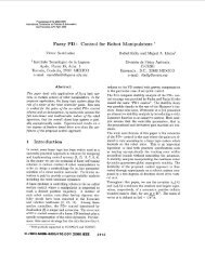
<strong>Nonlinear</strong> <strong>PID</strong> Control <strong>with</strong> Sliding<br />
Modes <strong>for</strong> Tkacking <strong>of</strong> Robot Manipulators<br />
V. <strong>Parra</strong>-Vega5 and S. Arimotot<br />
SMechatronics Division, CINVESTAV, AP 14-740, M6xic0, DF, Mdxico, vparra@mail.cinvestav.mx<br />
$Department <strong>of</strong> Robotics, Ritsumeikan Univ., 1-1-1 Noji-Higashi, Kusatsu, Shiga 525-8577, Japan.<br />
Abstmct-It is well-known that PI) <strong>control</strong>ler plus gravity<br />
compensation yields the global asymptotic stabllitjr <strong>for</strong> regdatiun<br />
tasks <strong>for</strong> <strong>robot</strong> <strong>manipulators</strong> [l], [a]. The impressive<br />
succew <strong>of</strong> these <strong>control</strong>lers in real-time tasks lie in the fact<br />
that they do neither compensate inertial nor coriolis <strong>for</strong>ces,<br />
so neither inertial nor coriolis matrices are needed to implement<br />
the <strong>control</strong>ler. However this linear state feedback <strong>control</strong>lers<br />
<strong>with</strong> gravity compeneation mnnot render asymptotic<br />
stability <strong>for</strong> tmcking tab. In this paper, a simple decentralized<br />
continuous nonlinear <strong>PID</strong> <strong>control</strong>ler that yields local<br />
exponential stability <strong>for</strong> <strong>tracking</strong> tasks is proposed. The<br />
<strong>control</strong>ler does neither need the inertial nor the Coriolis matrix.<br />
Comparative experimental data versus [l] and [SI <strong>for</strong><br />
a rigid mbot arm validates our design.<br />
Kegwd- <strong>PID</strong>, Sliding Mode Control, Robot Manipulators<br />
I. INTRODUCTION<br />
Studies on the <strong>control</strong> theory <strong>of</strong> serial mechanical SYStems<br />
have been subject <strong>of</strong> intensive and pr<strong>of</strong>itable research<br />
over the last two decades. In particular, industrial <strong>robot</strong><br />
prototypes have been <strong>control</strong>led poinbhpoint using the<br />
linear decentralized <strong>PID</strong> <strong>control</strong>lers <strong>with</strong>out gravity compensation.<br />
Most <strong>of</strong> these <strong>control</strong>lers have been designed using<br />
linear models, or linearized ones, and some interesting<br />
nonlinear <strong>PID</strong> structures have been proposed to overcome<br />
the limitations <strong>of</strong> traditional linear <strong>PID</strong> <strong>control</strong>lers <strong>for</strong> regulation<br />
tasks <strong>of</strong> nonlinear mechanical plants [4]-[ll]. The<br />
<strong>tracking</strong> capability <strong>of</strong> these <strong>control</strong> systems over the entire<br />
domain <strong>of</strong> the nonlinear dynamics is still a challenging<br />
research topic.<br />
A. Regulation<br />
The breakthrough PD <strong>control</strong>ler proposed by Takegaki<br />
and Arimoto in 1981 [l] paved the way to establiih theoretical<br />
foundations to <strong>control</strong>ling <strong>robot</strong>ic systems. The<br />
successful application <strong>of</strong> this <strong>control</strong>ler <strong>for</strong> regulation tasks<br />
in many physical systems becomes apparent because there<br />
are available explicit tuning procedures, as well as online<br />
compensation techniques <strong>of</strong> the gradient <strong>of</strong> the potential<br />
energy [6],[ll],[9],[7]. Recently <strong>PID</strong>-like <strong>control</strong>lers have<br />
been proposed which do not require La’SaUe’s arguments<br />
[4], [lo], however any <strong>of</strong> these <strong>control</strong>lers are not useful to<br />
obtain <strong>tracking</strong>. An outstanding mechatronic design together<br />
<strong>with</strong> a <strong>PID</strong>-like <strong>control</strong>ler may be good enough <strong>for</strong><br />
many <strong>robot</strong> based industrial applications. The success <strong>of</strong><br />
these kind <strong>of</strong> studies are driven by the simplicity and useful-<br />
ness <strong>of</strong> non-model based <strong>robot</strong> <strong>control</strong>lers. There<strong>for</strong>e, it is<br />
interesting the class <strong>of</strong> model-free decentralised <strong>control</strong>lers<br />
that can overcome some <strong>of</strong> the typical deficiencies <strong>of</strong> linear<br />
regulators but at the same time can render at least similar<br />
real time per<strong>for</strong>mance compared to some model-based<br />
<strong>tracking</strong> <strong>control</strong>lers [3].<br />
B. lhckang<br />
On the other hand, when model-based nonlinear <strong>control</strong><br />
law is designed, a complex nonlinear <strong>control</strong>ler is obtained,<br />
and typically no easy and no clear tuning procedures are<br />
proposed [13] except <strong>for</strong> some well-studied <strong>robot</strong>ic prote<br />
types in reaearch laboratories. In the laboratory, these <strong>control</strong>lers<br />
certainly yields high per<strong>for</strong>mance over the whole<br />
domain <strong>of</strong> the dynamical system but in the industrial floor<br />
the lack <strong>of</strong> tuning procedures and the high implement&<br />
tion and computational cost deprive us to fully obtain the<br />
advantages <strong>of</strong> model-based nonlinear <strong>control</strong>lers over the<br />
decentralized model-free linear <strong>control</strong>lers [13], [18], [19].<br />
C. Contribution<br />
In this paper, motivated by a mechatronics design, and<br />
considering the real-time per<strong>for</strong>mance <strong>of</strong> some nonlinear<br />
<strong>control</strong>lers, a new structure <strong>of</strong> a continuous nonlinear <strong>PID</strong><br />
<strong>control</strong> law <strong>for</strong> continuous mechanical plants <strong>with</strong> <strong>tracking</strong><br />
capability is proposed. The nonlinear I-tame <strong>control</strong><br />
input compensates <strong>for</strong> inertial, coriolis and gravitational<br />
<strong>for</strong>ces, while the PD action comprises <strong>for</strong> an stabilizer <strong>of</strong><br />
closed loop system trajectories. Experimental data d i -<br />
dates our design where, surprisingly enough, in some cases<br />
this model-free <strong>control</strong>ler yields better per<strong>for</strong>mance in comparison<br />
<strong>with</strong> the model-based adaptive <strong>control</strong>ler [3].<br />
In Section 11, it is presented the class <strong>of</strong> nonlinear systems<br />
considered in this article. Section I11 shows the <strong>control</strong><br />
law and presents its stability analysis, and Section lV<br />
discusses some aspects <strong>of</strong> the <strong>control</strong> structure. Section<br />
V shows the experimental set up and discusses the closedloop<br />
real-time per<strong>for</strong>mance. Finally, in Section VI some<br />
conclusions axe presented.<br />
11. NONLINEARDBOT DYNAMICS<br />
The dynamic model <strong>of</strong> a rigid n-link serial non-redundant<br />
<strong>robot</strong> manipulator <strong>with</strong> all actuated revolute joints de-<br />
Owe do not intend to <strong>of</strong>fer an extensive review on the subject <strong>of</strong><br />
nonlinear <strong>PID</strong> <strong>control</strong>ler, we review briefly the literature <strong>of</strong> a class <strong>of</strong><br />
passivity-based <strong>control</strong>lers <strong>for</strong> <strong>robot</strong> arms.<br />
0-7803-6733-2/01/$10.00 0 <strong>2001</strong> IEEE 351
scribed in joint coordinates is given as follows<br />
Wda + a 1414 + Bo4 + G(q) = 71 (1)<br />
where H(q) E Rnxn denotes a symmetric positive definite<br />
inertial matrix, BO E Rnxn stands <strong>for</strong> a diagonal positive<br />
definite matrix composed <strong>of</strong> damping friction coefficients<br />
€or each joint, C(q,q) E RnXn stands <strong>for</strong> the coriolis and<br />
centrifugal <strong>for</strong>ces, G(q) E 92" models the gravity <strong>for</strong>ces,<br />
and r E 8" stands <strong>for</strong> the torque input.<br />
A. Open Loop Emr Dynamics<br />
Since equation (1) is linearly parametrizable [3] by the<br />
product <strong>of</strong> a regressor Y = Y (q,cj,d,q) E RnxP, composed<br />
<strong>of</strong> known nonlinear functions, and a vector 8 E RP<br />
which represents unknown but constant parameters, then<br />
the parametrization Y8 can be written in terms <strong>of</strong> a nominal<br />
reference &, to be defined yet, and its derivative & as<br />
follows<br />
H(q)ir + (BO + C(qi 4)) 4r + G(Q) = Kei (2)<br />
where the regressor Yr = Yr (q, Q, Qrl Q) E Rnxp. Equ*<br />
tion (2) into (1) yields the open loop error dynamics in<br />
error coordinates S, as follows<br />
H(q)Sr + {BO + C(qi 4)) sr = * - Yre, (3)<br />
where Sr is defined by<br />
s, =q-q,. (4)<br />
Now, consider the following nominal reference qr and its<br />
derivative defined as follows 1131<br />
qr = qd - CUAq + Sd "/U, (5)<br />
b = wn(AS),<br />
where a, 7 are diagonal positive definite n x n matrices,<br />
function sgn(*) stands <strong>for</strong> the signum function <strong>of</strong> (*), and<br />
<strong>for</strong> IC<br />
AS = s-sd (6)<br />
S = AQ+aAq (7)<br />
sd = S(to)mp-'S(t-to) (8)<br />
> 0 and S(to) stands <strong>for</strong> S(t) at t = to. Notice<br />
that & = - aAq + & - ysgn(AS) k discontinuous, and<br />
AS(b) = 0 V <strong>for</strong> any initial condition. Equation (5) into<br />
(4) gives rise to the dynamic error coordinates<br />
Sr = AS + TU. (9)<br />
We now introduce some useful properties <strong>for</strong> the stability<br />
analysis.<br />
Properties: There exists positive scalars Pi, where i =<br />
0, ..., 5 such that<br />
2 Po > 0, &(A) 5 PI < 00 stand <strong>for</strong> the<br />
where X,(A)<br />
minimum and maximum eigenvalues <strong>of</strong> an A E Rnxn matrix,<br />
respectively. Norms IlAll = d-,<br />
and llbll <strong>of</strong><br />
vector b E Rn stand <strong>for</strong> the induced Frobenius and vector<br />
Euclidean norms, respectively. These constants can be<br />
computed from the state <strong>of</strong> the system, desired trajectories,<br />
feedback gains, and a conservative upper bounds <strong>of</strong> the dynamic<br />
model <strong>of</strong> the <strong>robot</strong> arm, besides that it is assumed<br />
that qd E c2.<br />
111. NONLINEAR <strong>PID</strong> CONTROLLER<br />
A decentralized model-free nonlinear <strong>PID</strong> <strong>control</strong>ler is<br />
stated in a theorem.<br />
Theorem 1: Consider the <strong>robot</strong> dynamics (1) in closed<br />
loop <strong>with</strong> the <strong>control</strong>ler given by:<br />
T = -Kdsr (11)<br />
t<br />
= -KpAq - K,Aq + KdSd - Ki 1 sgn(AS(F))&<br />
where sr is given in (Q), and Kd is a n X n diagonal symmetric<br />
positive definite matrix, and Kp = &a, K, = Kd,<br />
and Ki = &"/. Then, if error on initial condition are small<br />
enough, then local exponential <strong>tracking</strong> is assured provided<br />
that 7 in (9) is tuned accordingly to the inequality (21)<br />
given in the pro<strong>of</strong>.<br />
A. Stability Analysis<br />
Equation (11) into (3) renders the following closed-loop<br />
error dynamics<br />
H(q)Sr = - {K + C(q, 4)) sr - Yre (12)<br />
where K = Kd + Bo. A passivity-motivated analysis yields<br />
the following Lyapunov function<br />
whose total derivative along its solution (12) is given by<br />
V = -S,TKSr - S,'Yr8. (14)<br />
The norm <strong>of</strong> the function Yre in (12) is upper bounded<br />
according to the following derivations<br />
Yre 5 IIH(S)IIIISll+ II (BO + C(qi4))dr + llG(q)Il<br />
5 XM(H(q)) {allAdl +P6) $. {XM(BO)+<br />
+hlQI) (allAcrll+ P4 3- 7lloll) + P3<br />
5 Pl4lAQll + XMM(B0) + PzIlOll(~llAqI1+ P4 +<br />
+7Il4) +A<br />
5 +q, Ad1 a, Pi) (15)<br />
where ps = PIPS+& and v(Aq, A& a, A) is a scalar. Then<br />
according to (15), equation (14) becomes<br />
Q 5 -llK~sr112 + Ilsrllv(&,Aq,o,Pi) (16)<br />
where K = G Kl. Since Sr = v'(Aq,Aq,Sd,a), then if<br />
initial conditions me such that to) belongs to a compact<br />
tD<br />
352
set ne= the equilibrium S, = 0, we have that by invoking<br />
Lyapunav arguments, there exist 0 < K1 < 00 large enough<br />
such that S, converges into a neighborhood e > 0 <strong>with</strong><br />
radius r > 0 centered in the equilibrium S, = 0. Thus, the<br />
boundedness <strong>of</strong> S, can be concluded, namely<br />
Sr+Eo 89 t+W, (17)<br />
<strong>for</strong> a bounded constant EO, and €1 > 0 stands <strong>for</strong> the<br />
upper bound <strong>of</strong> S,. This result stands <strong>for</strong> local stability<br />
<strong>of</strong> Sr provided that the state is neax the desired trajectories<br />
<strong>for</strong> any initial conditions. Thus, boundedness <strong>of</strong><br />
S, = q'(Aq, Aq, sd, .) together <strong>with</strong> boundedness <strong>of</strong> feedback<br />
gains and desired trajectories imply the boundedness<br />
<strong>of</strong> Deltaq, Aq, sd, 6, and there<strong>for</strong>e the boundedness <strong>of</strong> Y,Q.<br />
In virtue that H(q) %,positive dehite, we can also conclude<br />
the boundedness <strong>of</strong> Sr as follows<br />
s, = -H(q)-l {(K + C(q, q))sr - &e}<br />
I h(H(Q)-l) {(hm + P211~11)~1+ 9)<br />
I C(Q9 Q, dA4, Ad, 4) (18)<br />
where the bounded function
which yields<br />
t<br />
Sr=AS+TLAS(C)e& (25)<br />
where AS and s d are given in (7)-(9), and a, dd = 2j + 1,<br />
j are non-negative integer. Then, a continuous terminal<br />
attractor is induced in finite time provided that 7 in (9) is<br />
tuned according to (21). A<br />
In equation (25), the coefficients dn and dd give ad&-<br />
tiond degrees <strong>of</strong> freedom to shape the dynamic surface S,.<br />
Surface (25) together <strong>with</strong> <strong>control</strong> (11) yields fast asymp<br />
totic convergence <strong>with</strong> a certain degree <strong>of</strong> robustness (see<br />
Figure 5).<br />
On the other hand, several interesting results have been<br />
obtained by using saturated filtered errors ([ll],[4]. These<br />
schemes basically introduce timevarying feedback gains,<br />
among other technicd advantages.<br />
Pmpsition 3: Consider the <strong>robot</strong> dynamics (1) in closed<br />
loop <strong>with</strong> the <strong>control</strong>ler (ll), provided that y in (9) is tuned<br />
according to (21) the we have the following:<br />
Hyperbolac Tangent.<br />
Consider the following dynamic change <strong>of</strong> coordinates using<br />
qr = qd-atanh(A&) +sdl-Tlsql(r)e&<br />
AS = & + a tanh(XAq) - S ~(to)~-"(~-~)<br />
I<br />
-' *<br />
s1<br />
sd I<br />
Then, a wntinuous saturated terminal attractor is induced<br />
in finite time.<br />
Satunrted Sine.<br />
Consider the following dynamic change <strong>of</strong> coordinates<br />
t<br />
Qr = qd - crSin(AAq) f Sd2 - 7 lo AS(c)%d<<br />
AS = Aq + aSin(XAq) - Sz(t~)ezp-"(~-~~)<br />
-'<br />
t<br />
Sa<br />
SdZ<br />
t<br />
sr = AS + 7 J, AS(~)%~C (27)<br />
A. Hardware<br />
A two degrees <strong>of</strong> freedom direct drive ShinMaywa R3C<br />
<strong>robot</strong> arm is used as testbed. It is a rigid-link, low-friction,<br />
planar <strong>robot</strong> <strong>with</strong> two joints. Dimensions <strong>of</strong> the <strong>robot</strong><br />
are given in Table I, where subindex 1 and 2 stand <strong>for</strong><br />
first and second link, respectively, and L, stands <strong>for</strong> the<br />
center <strong>of</strong> mass, Pur means parameters, I stands <strong>for</strong> inertia,<br />
and A defines joint limits. Joint position is measured<br />
<strong>with</strong> optical encoders <strong>with</strong> resolution <strong>of</strong> 120,000 pulselrad<br />
and joint velocity signal is estimated from position signals<br />
using a first order filter <strong>with</strong> a constant T = 10.0.<br />
Viscous friction damping coefficients were estimated using<br />
an adaptive <strong>control</strong>ler <strong>with</strong> persistent exciting trajectories<br />
[3] running during 5min to obtain nominal coefficients are<br />
Bo = (B11 = 1.674, B22 = 1.472)Nms.<br />
B. Firmware<br />
A Digital Signal Processor Loughborough Sound Images<br />
Ltd DPCIC40B board <strong>control</strong> system was integrated on<br />
a 16bit expansion bus slot <strong>of</strong> a DX - 486 personal computer.<br />
TMS320 floating point DSP C v.1.0.1 compiler provided<br />
the programing environment. The <strong>control</strong> input is<br />
transmitted to the servomotors through the Shmmaywa<br />
servosystem which powers the pulse wide modulators motor<br />
drives at each joint.<br />
C. Experimental Data<br />
The per<strong>for</strong>mance <strong>of</strong> the proposed <strong>control</strong>ler is shown in<br />
comparison to the standard PD [l] and the baseline modelbased<br />
adaptive <strong>control</strong>ler [3]. Experiments are carried out<br />
at high velocities in order to show the per<strong>for</strong>mance <strong>of</strong> the<br />
system at inertial dominated dynamics.<br />
C.1 Initial conditions, desired trajectories, and gains<br />
Desired trajectories at each joint are Qd(t) =<br />
AX:=, sin (7) where A = $! deg/rad is the amplitude<br />
and fm = 5 s and fn = 2.5 S, <strong>for</strong> middle and high<br />
velocities respectively, stands <strong>for</strong> the period. The irequencies<br />
w, are w1 = 1.0 Ha, w2 = 2.0 Hz and w3 = 4.0 Hz.<br />
The peak desired velocity is 87.96 deg/s and the peak desired<br />
acceleration is 304.64 deg/s2. Initial conditions are<br />
set about -5.0 deg <strong>with</strong> zero initial velocity. Feedback<br />
gains are given in the "able 11.<br />
Then, a continuous saturated terminal attractor is induced.<br />
A<br />
Surface (26) and (27) yield fast asymptotic convergence<br />
<strong>with</strong> a certain degree <strong>of</strong> robustness. Since the system is<br />
very sensitive to the feedback gain a, the tuning <strong>of</strong> X can<br />
improve signiscantly the response <strong>of</strong> the closed-loop system,<br />
(see Figure 7).<br />
V. EXPERIMENTAL RESULTS<br />
In this section the experimental setup and then the experimental<br />
data is discussed and analyzed.<br />
C.2 Tuning <strong>control</strong> gains<br />
Wing the parameters is nothing obvious and special attention<br />
is paid to avoid misleading conclusions. Since we<br />
Par I( Mass I Lank I L, ( I ( A<br />
DOFl II 21.20 I 0.25 I 0.15 I 0.21 I f160<br />
DOF;<br />
Units<br />
15.22 0.45 0.19 0.18 A145<br />
Kg n m Kgm2 deg<br />
354
TABLE 11<br />
FEEDBACK GAINS<br />
present a comparison among similar but structurally Merent<br />
<strong>control</strong>lers, we set common gains to the same value, see<br />
Table 11, where values stand <strong>for</strong> the diagonal entry times<br />
an identity matrix <strong>of</strong> proper dimensions, and w,, stands <strong>for</strong><br />
the desired natural frequency and T) the damping ration <strong>of</strong><br />
the PD <strong>control</strong>ler [l].<br />
c.3 Results<br />
Comparative experiments are difficult to obtain because<br />
any comparative result can be biased dangerously, besides<br />
that it is difficult to compare qualitatively <strong>control</strong>lers that<br />
are structurally Werent. To this end, we have limited our<br />
study to pasivity based <strong>control</strong>lers [3], [l], and [2] that have<br />
some common gains. We show experimental results obtained<br />
”at kst run”, that is when reasonable per<strong>for</strong>mance,<br />
as dictated by the theory, is obtained <strong>with</strong>out perhaps obtaining<br />
the best plots. Surprisingly enough, in all cases our<br />
<strong>control</strong>ler outper<strong>for</strong>ms 131. To have a better view on the<br />
results some plots are shown in two windows.<br />
Figure 1 shows a comparative plot <strong>of</strong> positions <strong>tracking</strong><br />
errors at high velocities <strong>of</strong> the <strong>control</strong>lers <strong>PID</strong> 111, and our<br />
Sliding-PD <strong>control</strong>. After a transient <strong>of</strong> 1 s, our <strong>control</strong>ler<br />
respect to [Z] yields <strong>tracking</strong> errors at each joint <strong>of</strong> threefold<br />
and fourteenfold smaller respectively,<br />
Figure 3 depicts the establishment <strong>of</strong> a terminal attractor<br />
at AS = 0 <strong>of</strong> <strong>control</strong> (11) and (26). When % = 1.0 we<br />
have in fact a PI <strong>control</strong>ler in the error space AS. When<br />
& < 1.0 a terminal attractor or slider is induced at AS =<br />
0. Figure 4 shows <strong>control</strong> and position <strong>tracking</strong> errors when<br />
we use Sliding-PD <strong>control</strong> <strong>for</strong> Werent dues <strong>of</strong> K in sd.<br />
We can see that by simply tuning K we can slow down or<br />
speed up the response <strong>of</strong> the system. Figure 5 shows the<br />
effects <strong>of</strong> setting different values <strong>of</strong> saturation, via X in (26).<br />
The higher the X the faster the response and the smaller<br />
<strong>tracking</strong> errors.<br />
Figure 6 shows comparative results between the <strong>control</strong>ler<br />
Sliding-PD and [3] where we can o k e that our<br />
<strong>control</strong>ler yields better <strong>tracking</strong> accuracy <strong>with</strong> smooth <strong>control</strong><br />
input, even when (31 started <strong>with</strong> smaller position<br />
trackiig errors. It has been set the maximum feedback<br />
<strong>control</strong> gains that [3] can af<strong>for</strong>d <strong>with</strong>out going into stability<br />
or saturated problems.<br />
VI. CONCLUSIONS<br />
An approach to <strong>control</strong> a class <strong>of</strong> <strong>robot</strong> <strong>manipulators</strong> using<br />
a very simple decentralized model-free <strong>PID</strong> <strong>control</strong>ler<br />
has been proposed. Experimental data shows the per<strong>for</strong>mance<br />
<strong>of</strong> the proposed <strong>control</strong>ler where it is concluded the<br />
vaIidity <strong>of</strong> the proposed scheme. In this particular experimental<br />
set-up, our model-free decentrdi <strong>control</strong>ler af-<br />
<strong>for</strong>ds at least similar per<strong>for</strong>mance compared to the modelbased<br />
adaptive <strong>control</strong>ler [3] <strong>for</strong> <strong>tracking</strong> tasks.<br />
ACKNOWLEDGMENTS<br />
The authors acknowledge the anonymous reviewers <strong>for</strong><br />
their helpful comments. This work was carried out under<br />
the Japan Society <strong>for</strong> Promotion <strong>of</strong> Science and the<br />
Institute <strong>for</strong> Transfer <strong>of</strong> Industrial Technology Fellowships<br />
<strong>of</strong> Japan, and written during an Alexander von Humboldt<br />
Fellowship in the Institute <strong>for</strong> Roboticas and Mechantronics,<br />
Germany, all held by the first author.<br />
REFERENCES<br />
‘palaegaki M. and Arimoto S. “A New Feedback Method <strong>for</strong> Dynamic<br />
Control <strong>of</strong> Manipulators”, Journal <strong>of</strong> Dyamic Systems,<br />
Mmmenta, and Control, voL103, June 1981.<br />
Arimoto S. and Miyazaki F., UStability and Robustness <strong>of</strong> a <strong>PID</strong><br />
Feedback Control <strong>for</strong> Robot Manipulstors <strong>of</strong> Sensory Capabilities,”<br />
Robotics Rmeamh: First International Symposium, M.<br />
Brady and R.P. Paul eds., Boston:MIT Press, 1984.<br />
Slotine J. J. and Li W., ”On the Adaptive Control <strong>of</strong> Manipulators”,<br />
Intffnationl Journal <strong>of</strong> Robotics Reaeamh, vo1.6, No. 3,<br />
pp. 49-59, 1987.<br />
S. Arimoto, T. Naniwa, V. <strong>Parra</strong>-Vega, and L.L. Whitcomb,<br />
A Natural PD Control <strong>for</strong> Robot Manipulators and its Role in<br />
Adaptive and Learning Controls,” S<strong>of</strong>t Computing, Ignaural Is<br />
sue, 1995.<br />
H. G. Sagq M. F. De Mathelin, E. Ostertag, “Robust <strong>control</strong> <strong>of</strong><br />
<strong>robot</strong> <strong>manipulators</strong>: a survey“, International Journal <strong>of</strong> Control,<br />
1999.<br />
Voda A.A. and Landau I.D., “A Method <strong>for</strong> the Calibration <strong>of</strong><br />
<strong>PID</strong> Controllers,” Automaticq 1995, Vo1.31, No.1, pp. 35-53.<br />
Tomei P., “Adaptive PD <strong>for</strong> Robot Manipulators,” IEEE Iltumaactions<br />
<strong>of</strong> Robotics and Automation, Vo1.7, N0.4, August 1991.<br />
Hsia T.C., “Robustness Analysia <strong>of</strong> a PD Controller <strong>with</strong> Ag<br />
proximante Gravity Compensation <strong>for</strong> Robot Manipulators,”<br />
Jouml <strong>for</strong> Robotic8 Systems, Vol.11, N0.6, 1994.<br />
S.M. Shahruz, G. Langari and M. Tomizuka, “Design <strong>of</strong> Robust<br />
PD-type Control Laws <strong>for</strong> Robot Manipulators <strong>with</strong> Parametric<br />
Uncertainties,” Journal <strong>for</strong> Robotics Systems, Vol.10, No.4,1993.<br />
R Kelly, “A Tuning Procedure <strong>for</strong> <strong>PID</strong> Control <strong>for</strong> Robot Manipulators,”<br />
Submitted <strong>for</strong> review to the IEEE Il)ansactions on<br />
Robotics and Automation<br />
V. Santibanez and R. Kelly, “Strict Lyapunov Functions <strong>for</strong><br />
Global Regulation <strong>of</strong> Robots Manipulators,” ZEEE International<br />
Conference on Robotics and Automation, Nagoya, Japan, 1995.<br />
Y. Stepanenko, Yong Cao, and Chun-Yi Su, “Variable Structure<br />
Control <strong>of</strong> Robotic Manipulator <strong>with</strong> <strong>PID</strong> Sliding Surfaces,” Int.<br />
Journal <strong>of</strong> Robust and <strong>Nonlinear</strong> Control, Vol. 8, pp. 79-90,<br />
1998<br />
Vicente <strong>Parra</strong>-Vega and Suguru Arimoto, ”Adaptive Control <strong>for</strong><br />
Robot Manipulators <strong>with</strong> Sliding Mode Error Coordinate System:<br />
Free and Constrained Motions,” IEEE International Conference<br />
on Robotics and Automation, Nagoya, Japan, 1995.<br />
Utkin V., Variable Structure Systems: Contml and Optamixatian,<br />
1992<br />
Tarokh, M, Decoupled <strong>Nonlinear</strong> Three-lbrm Controllers <strong>for</strong><br />
Robot Dajectory Daclcing, IEEE Zhnsactions on Robotics and<br />
A~tomation, 1999,152,369 - 380.<br />
Seraji, Homayoun, A New Class <strong>of</strong> <strong>Nonlinear</strong> <strong>PID</strong> Controllers<br />
<strong>with</strong> Robotic Applications, Journal <strong>of</strong> Robotic Systems, 1998,<br />
15-3, 161.<br />
Wijerroma, W S; Kodagoda, K R S, Synthesis <strong>of</strong> Stable Fuzzy<br />
PD/<strong>PID</strong> Control Laws <strong>for</strong> Robotic Manipulators from a Variable<br />
Structure Systems Standpoint, Lecture Notes in Computer<br />
Science, 1999, 1625,495 - 511.<br />
R Kelly, Global Positioning <strong>of</strong> Robot Manipulators via PD Control<br />
Plus A Class <strong>of</strong> <strong>Nonlinear</strong> Integral Actions, IEEE Thansactim<br />
an Automatic Control, 1998,43-7,934 - 937.<br />
Pervozva~ki, Anatoli A.; Reidovich, Leonid B., Robust Stabilization<br />
<strong>of</strong> Robotic Manipulators by <strong>PID</strong> Controllers, Dynamics<br />
and Control, 1999,9-3, 203 - 222.<br />
35s
<strong>PID</strong> VB SAdlno-m. TreownO lntwowlndova Trackingem~sandconm~l vsluesol hSd<br />
4 1 : : - . .<br />
...... .......,... .:.... ..............<br />
.........<br />
............<br />
.............<br />
. . .<br />
0.6 1 t 2 3 4 6 -100. , 2 4 -10 2 4<br />
6<br />
wlndov 1 WinQw2 rime[] nme[sl<br />
......<br />
......<br />
. , .<br />
2 : . .<br />
. ._ ..<br />
......<br />
nme [ai<br />
.................<br />
. . .<br />
. . . .<br />
5 2 3 4 5<br />
n-m IO1<br />
Fig. 1. Gomparative wormance between [2] and our Controller (12)<br />
in terms <strong>of</strong> position <strong>tracking</strong> errors. Dash line stands <strong>for</strong> <strong>PID</strong> 111<br />
and solid line stands <strong>for</strong> our <strong>control</strong>ler.<br />
4 6<br />
nma [sj<br />
............ i ............ j .............<br />
-200 2 4<br />
nms [si<br />
Fig. 4. Per<strong>for</strong>mance <strong>of</strong> Sliding-PD <strong>control</strong> <strong>for</strong> different values <strong>of</strong> n<br />
(n = 1.0(.), = 5.0(.-), = io.o~), = 20.0(-)).<br />
gldllrg<strong>modes</strong>lnbcsdbye Beturatsd IOdar-PD Gonvol SPolmW sM.r-PD ccnool trsckkgermklw0WtndOIYB<br />
0.04<br />
0.1<br />
................... ...................<br />
................... .:....................<br />
......<br />
............ 2 -0.05<br />
-8<br />
-0.1<br />
0.5<br />
Wlndorrl wlndow 1 Window2<br />
rime 181<br />
. .<br />
:<br />
-0.1 . : -<br />
1 2 3 4 5<br />
IS1<br />
Fig. 2. Sliding <strong>modes</strong> are established in leas than 1 s using <strong>sliding</strong>- Fig. 5. per<strong>for</strong>mance <strong>of</strong> saturated error manifolds, using Sin(%) <strong>for</strong><br />
'<br />
PD <strong>control</strong>ler (12). differat values Of A (A = l.O(.), A = 5.0(-.), A = lO.O(:)).<br />
-noPo<br />
(r) VI slot a U*@)<br />
2 ................ .:_ ................<br />
P-<br />
-Om<br />
.-A ........ .............................<br />
E' ;'<br />
2, .............. I.. ..........<br />
-80 0.5 1<br />
Whdarl<br />
4f & ............... .:...................<br />
N -4 ......<br />
p 3'-<br />
4-e .............. :...................<br />
-a<br />
0.5<br />
Tbne I4<br />
I<br />
O ;....... 2t .I.......... -*.. R<br />
0.1 .........<br />
. . .<br />
0 ..............<br />
. . .<br />
. .<br />
-03'1 2 3 4 5<br />
-me[SI<br />
-1 5<br />
..,.. i ...................<br />
0.5<br />
Wndavl<br />
...................<br />
..................<br />
7-10 ..................<br />
-1 5<br />
0.5<br />
1<br />
1<br />
Fig. 3. TraEking errors using terminal attractors at As = 0 (20) <strong>for</strong> Fig. 6. Comparative result <strong>of</strong> Slotine and Li and <strong>Nonlinear</strong> <strong>PID</strong>:<br />
different values <strong>of</strong>ratio 2 (E(-.), E(:), %(-I, &(.I). "k.acking errom in two windows.<br />
356