Quantum error correction and fault-tolerant quantum computation
Quantum error correction and fault-tolerant quantum computation
Quantum error correction and fault-tolerant quantum computation

Create successful ePaper yourself
Turn your PDF publications into a flip-book with our unique Google optimized e-Paper software.
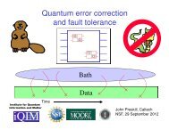
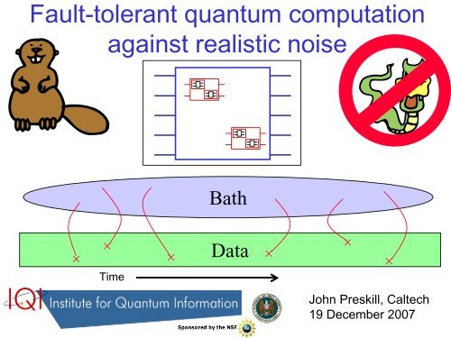
Fault-<strong>tolerant</strong> <strong>quantum</strong> <strong>computation</strong><br />
against realistic noise<br />
Bath<br />
×<br />
× × Data ×<br />
Time<br />
×<br />
×<br />
John Preskill, Caltech<br />
19 December 2007
<strong>Quantum</strong> <strong>fault</strong> tolerance<br />
• Error <strong>correction</strong> <strong>and</strong> <strong>fault</strong> tolerance will be essential in the<br />
operation of large-scale <strong>quantum</strong> computers, both to prevent<br />
decoherence <strong>and</strong> to control the cumulative effects of small<br />
<strong>error</strong>s in unitary <strong>quantum</strong> gates.<br />
• This talk focuses on <strong>fault</strong>-<strong>tolerant</strong> processing of <strong>quantum</strong><br />
information using <strong>quantum</strong> <strong>error</strong>-correcting codes (the<br />
foundation for our belief that scalable <strong>quantum</strong> computers are<br />
possible).<br />
• There are a variety of other useful ideas concerning protecting<br />
<strong>quantum</strong> computers from noise … e.g., dynamical decoupling,<br />
noiseless subsystems, protection arising from (nonabelian)<br />
topological order, …<br />
• I won’t say much about these other ideas, even though they<br />
are important, they are related to my main topic, <strong>and</strong> they can be<br />
fruitfully combined with the methods I’ll discuss.
Fault-<strong>tolerant</strong> <strong>quantum</strong> <strong>computation</strong><br />
1. Fault-<strong>tolerant</strong> <strong>quantum</strong> computing<br />
2. <strong>Quantum</strong> accuracy threshold theorem<br />
3. Biased noise (Aliferis-Preskill 2007)<br />
4. Non-Markovian (Gaussian) noise.
Fault tolerance<br />
<strong>Quantum</strong> information can be protected by a <strong>quantum</strong> <strong>error</strong>correcting<br />
code. But the <strong>quantum</strong> gates that we use to encode<br />
<strong>and</strong> to recover from <strong>error</strong> are themselves noisy.<br />
• The measured <strong>error</strong> syndrome (i.e., the eigenvalues of the<br />
check operators) might be inaccurate.<br />
• Errors might propagate during syndrome measurement.<br />
• We need to implement a universal set of <strong>quantum</strong> gates that<br />
act on encoded <strong>quantum</strong> states, without unacceptable <strong>error</strong><br />
propagation.<br />
• We need codes that can correct many <strong>error</strong>s in the code block.
Fault-<strong>tolerant</strong> <strong>error</strong> <strong>correction</strong><br />
Fault: a location in a circuit where a gate or storage <strong>error</strong> occurs.<br />
Error: a qubit in a block that deviates from the ideal state.<br />
X<br />
Error<br />
Correction<br />
Error<br />
Correction<br />
X<br />
X<br />
If input has at most one <strong>error</strong>, <strong>and</strong><br />
circuit has no <strong>fault</strong>s, output has no<br />
<strong>error</strong>s.<br />
If input has no <strong>error</strong>s, <strong>and</strong> circuit has at<br />
most one <strong>fault</strong>, output has at most one<br />
<strong>error</strong>.<br />
Error<br />
Correction<br />
Error<br />
Correction<br />
X<br />
Error<br />
X<br />
Correction<br />
A <strong>quantum</strong> memory fails only if two <strong>fault</strong>s occur in some “extended rectangle.”
Fault-<strong>tolerant</strong> <strong>quantum</strong> gates<br />
Fault: a location in a circuit where a gate or storage <strong>error</strong> occurs.<br />
Error: a qubit in a block that deviates from the ideal state.<br />
X<br />
<strong>Quantum</strong><br />
Gate<br />
X<br />
<strong>Quantum</strong><br />
Gate<br />
X<br />
X<br />
If input has at most one <strong>error</strong>, <strong>and</strong><br />
circuit has no <strong>fault</strong>s, output has at most<br />
one <strong>error</strong> in each block.<br />
If input has no <strong>error</strong>s, <strong>and</strong> circuit has at<br />
most one <strong>fault</strong>, output has at most one<br />
<strong>error</strong> in each block.<br />
Error<br />
Correction<br />
<strong>Quantum</strong><br />
Gate<br />
X<br />
X<br />
Error<br />
Correction<br />
<strong>Quantum</strong><br />
Gate<br />
Each gate is preceded by an <strong>error</strong> <strong>correction</strong> step. The circuit<br />
simulation fails only if two <strong>fault</strong>s occur in some “extended rectangle.”
Fault-<strong>tolerant</strong> <strong>quantum</strong> gates<br />
Error<br />
Correction<br />
<strong>Quantum</strong><br />
Gate<br />
X<br />
X<br />
Error<br />
Correction<br />
<strong>Quantum</strong><br />
Gate<br />
Each gate is followed by an <strong>error</strong> <strong>correction</strong> step. The circuit<br />
simulation fails only if two <strong>fault</strong>s occur in some “extended rectangle.”<br />
If we simulate an ideal circuit with L <strong>quantum</strong> gates, <strong>and</strong> <strong>fault</strong>s occur<br />
independently with probability ε at each circuit location, then the probability of<br />
failure is<br />
2<br />
P ≤ LA ε<br />
fail<br />
max<br />
where A max is an upper bound on the number of pairs of circuit locations in each<br />
extended rectangle. Therefore, by using a <strong>quantum</strong> code that corrects one <strong>error</strong><br />
<strong>and</strong> <strong>fault</strong>-<strong>tolerant</strong> <strong>quantum</strong> gates, we can improve the circuit size that can be<br />
simulated reliably to L=O(ε −2 ), compared to L=O(ε −1 ) for an unprotected<br />
<strong>quantum</strong> circuit.
Recursive simulation<br />
In a <strong>fault</strong>-<strong>tolerant</strong> simulation, each (level-<br />
0) ideal gate is replaced by a 1-Rectangle:<br />
a (level-1) gate gadget followed by (level-<br />
1) <strong>error</strong> <strong>correction</strong> on each output block.<br />
In a level-k simulation, this replacement is<br />
repeated k times --- the ideal gate is<br />
replaced by a k-Rectangle.<br />
A 1-rectangle is built<br />
from <strong>quantum</strong> gates.<br />
A 2-rectangle is built<br />
from 1-rectangles.<br />
A 3-rectangle is built<br />
from 2-rectangles.<br />
(1) The <strong>computation</strong> is accurate if the <strong>fault</strong>s in a level-k simulation are sparse.<br />
(2) A non-sparse distribution of <strong>fault</strong>s is very unlikely if the noise is weak.<br />
There is threshold of accuracy. If the <strong>fault</strong> rate is below the threshold, then an<br />
arbitrarily long <strong>quantum</strong> <strong>computation</strong> can be executed with good reliability.
Level Reduction: “coarse-grained” <strong>computation</strong><br />
Simulated gate is correct if:<br />
gate gadget<br />
<strong>error</strong> <strong>correction</strong><br />
imaginary<br />
ideal decoder<br />
imaginary<br />
ideal gate<br />
propagate<br />
decoders to<br />
the left<br />
Simulated measurements<br />
<strong>and</strong> preparations<br />
are correct if:<br />
create<br />
decoders<br />
annihilate<br />
decoders<br />
Decoders sweeping from right to left transform a level-1 <strong>computation</strong> to an<br />
equivalent level-0 <strong>computation</strong>. Each “good” level-1 extended rectangle (with no<br />
more than one <strong>fault</strong>) becomes an ideal level-0 gate, <strong>and</strong> each “bad” level-1<br />
extended rectangle (with two or more <strong>fault</strong>s) becomes a <strong>fault</strong>y level-0 gate. If our<br />
noise model is stable under level reduction, the coarse-graining can be repeated<br />
many times.
Local Stochastic Noise<br />
space<br />
time<br />
Noisy Circuit = Σ “Fault Paths”<br />
For local stochastic noise with strength ε , the sum of the probabilities<br />
of all <strong>fault</strong> paths such that r specified gates are <strong>fault</strong>y is at most ε r .<br />
(For each <strong>fault</strong> path, the operations at the <strong>fault</strong>y locations are chosen by the<br />
adversary.)<br />
After one level reduction step, the circuit is still subject to local stochastic<br />
noise with a “renormalized” strength:<br />
ε ≤ ε / ε = ε ( ε / ε )<br />
(1) 2 2<br />
0 0 0<br />
The constant ε 0 is estimated by counting the number of “malignant” pairs of<br />
<strong>fault</strong> locations that can cause a 1-rectangle to be incorrect. If level reduction<br />
is repeated k times, the renormalized strength becomes:<br />
ε < ε ( ε / ε ) k<br />
( k ) 2<br />
0 0
Accuracy Threshold<br />
<strong>Quantum</strong> Accuracy Threshold Theorem: Consider a<br />
<strong>quantum</strong> computer subject to local stochastic noise with<br />
strength ε . There exists a constant ε 0 >0 such that for a fixed ε<br />
< ε 0 <strong>and</strong> fixed δ > 0, any circuit of size L can be simulated by a<br />
circuit of size L* with accuracy greater than 1-δ, where, for<br />
some constant c,<br />
( )<br />
L* = O⎡L logL<br />
⎤ ⎣ ⎦<br />
The numerical value of the accuracy threshold ε 0 is of practical<br />
interest!<br />
assuming:<br />
ε 0 > 2.73 × 10 -5<br />
parallelism, fresh ancillas (necessary assumptions)<br />
c<br />
Aharonov, Ben-Or (1996)<br />
Kitaev (1996)<br />
nonlocal gates, fast measurements, fast <strong>and</strong> accurate classical<br />
processing, no leakage (convenient assumptions).<br />
Aliferis,<br />
Gottesman,<br />
Preskill (2005)<br />
Reichardt (2005)
Some noteworthy recent developments<br />
1) Threshold for local gates in 2D – Svore, DiVincenzo, Terhal<br />
(2006)<br />
2) Threshold when measurements are slow – DiVincenzo,<br />
Aliferis (2006)<br />
3) Improved thresholds with subsystem codes – Aliferis,<br />
Cross (2006)<br />
4) Threshold for postselected <strong>computation</strong> – Knill (2004),<br />
Reichardt (2006), Aliferis, Gottesman, Preskill (2007)<br />
5) Improved threshold via flagging <strong>and</strong> message passing –<br />
Knill (2004), Aliferis (2007)<br />
6) Topological protection with cluster states – Raussendorf,<br />
Harrington, Goyal (2005, 2007)<br />
Rigorous threshold estimate for local stochastic noise:<br />
ε 0 > 1.0 × 10 -3
Two issues<br />
1) The local stochastic noise model describes generic noise<br />
with no special structure. Can we improve the threshold<br />
estimate by exploiting the structure of the noise in actual<br />
devices?<br />
2) The local stochastic noise model is h<strong>and</strong>y for analysis <strong>and</strong><br />
has some quasi-realistic features, but still rather artificial;<br />
as usually formulated it is not founded on a physical (e.g.<br />
Hamiltonian) description of the origin of the noise. Can we<br />
prove threshold theorems for noise models that are better<br />
motivated physically, <strong>and</strong> how is the numerical value of the<br />
threshold affected by coherence <strong>and</strong> memory in the<br />
interaction with the environment?
Biased Noise<br />
Aliferis-Preskill 2007<br />
In many physical settings, Z noise (dephasing) is much<br />
stronger than X noise (relaxation). Dephasing arises from<br />
low frequency noise, while relaxation arises from noise with<br />
frequency ~w 0 (the energy splitting between <strong>computation</strong>al<br />
basis states). Typically, the higher-frequency noise has a<br />
different physical origin than the low-frequency noise, <strong>and</strong> it<br />
can be orders of magnitude weaker.<br />
ω 0<br />
|1〉<br />
| 0〉<br />
Can <strong>fault</strong>-<strong>tolerant</strong> gadgets exploit this bias? We should use a code that<br />
corrects more Z <strong>error</strong>s than X <strong>error</strong>s (for example, a phase-<strong>error</strong> correcting<br />
repetition code at the bottom of a concatenated scheme). But our universal<br />
set of gate gadgets must have the property that the (common) Z <strong>error</strong>s do<br />
not propagate to become (rare) X <strong>error</strong>s. (For example, transversal<br />
Hadamard gates should be avoided.)<br />
X<br />
Z
Biased Noise<br />
Our universal set of gadgets must have the property that the (common) Z<br />
<strong>error</strong>s do not propagate to become (rare) X <strong>error</strong>s. For example, transversal<br />
Hadamard gates should be avoided. E.g., CNOT gates (which are<br />
transversal for CSS codes) do not propagate Z to X, <strong>and</strong> other gates in the<br />
universal set can be teleported. We could estimate the threshold under the<br />
assumption that CNOT gates have highly biased noise (Gourlay &<br />
Snowdon 2000, Stephens et al. 2007, Evans et al. 2007).<br />
But is it reasonable to assume that the CNOT gate has<br />
highly biased noise? Gates are realized by a timedependent<br />
control Hamiltonian that turns on <strong>and</strong> off,<br />
<strong>and</strong> a Z <strong>error</strong> occuring while a qubit is rotating on the<br />
Bloch sphere can generate an X <strong>error</strong>. Furthermore, if<br />
a qubit is rotated about the X axis, then an overrotation<br />
or under-rotation can generate an X <strong>error</strong>.<br />
We should distinguish between diagonal gates (diagonal matrices in the<br />
<strong>computation</strong>al basis) <strong>and</strong> nondiagonal gates; it is reasonable to assume<br />
that the noise in diagonal gates is dominated by dephasing, while the<br />
noise in nondiagonal gates has no spectial structure. For diagonal gates,<br />
the ideal control Hamiltonian commutes with Z at all times; these gates do<br />
not propapagate Z noise to X noise.
Local Stochastic Biased Noise Model<br />
Noisy Circuit = Σ “Fault Paths”<br />
In our biased noise model, there are two different values of the noise<br />
strength: ε quantifies the rate for dephasing <strong>fault</strong>s in diagonal gates <strong>and</strong> for<br />
unstructured <strong>fault</strong>s in non-diagonal gates, <strong>and</strong> ε ′
Fault-<strong>tolerant</strong> scheme<br />
We will build our <strong>fault</strong>-<strong>tolerant</strong> scheme using single-qubit preparations of the<br />
X eigenstate |+Ú = (|0Ú + |1Ú) /◊2, single-qubit measurements in the X basis, <strong>and</strong> the<br />
diagonal two-qubit CPHASE gate:<br />
CPHASE = controlled-Z = diag(1, 1, 1, -1)<br />
The n-qubit repetition code 1<br />
will protect against dephasing (Z <strong>error</strong>s) at the<br />
lowest level of a concatenated scheme, but it provides no protection against<br />
bit flips (X <strong>error</strong>s). Using our fundamental operations, we will construct a <strong>fault</strong><strong>tolerant</strong><br />
CNOT gate <strong>and</strong> <strong>fault</strong>-<strong>tolerant</strong> encoded measurements, where the<br />
effective noise in the encoded CNOT is approximately balanced. Then<br />
we may use well-known <strong>fault</strong>-<strong>tolerant</strong> constructions <strong>and</strong> a concatenated code<br />
2<br />
to realized highly accurate encoded CNOT gates protected by 1<br />
@ 2.<br />
Finally, we use injection by teleportation of the states<br />
|+iÚ = (|0Ú + i|1Ú) /◊2 |TÚ = (|0Ú + e iπ/4 |1Ú) /◊2<br />
<strong>and</strong> state distillation to complete the set of universal gadgets at the top level.<br />
highly biased noise<br />
{ CPHASE, P , M }<br />
| +〉<br />
{ P , P }<br />
| +〉 i | T〉<br />
σ<br />
x<br />
C 1<br />
more balanced<br />
effective noise<br />
G<br />
L<br />
CSS<br />
C 2<br />
G CSS<br />
very weak<br />
effective noise<br />
G universal<br />
injection <strong>and</strong><br />
distillation
Encoded Preparations <strong>and</strong> Measurements<br />
To be specific, consider the three-qubit repetition code (though we may<br />
actually want to use a longer code). The codewords are |+++Ú <strong>and</strong> |- - -Ú;<br />
these can be encoded <strong>and</strong> measured transversally:<br />
P |+〉<br />
P =<br />
|<br />
|+〉 L<br />
P |+〉<br />
P |+〉<br />
M σ x<br />
P<br />
x<br />
L<br />
M =<br />
|+〉 σ<br />
M σ x<br />
M σ x<br />
For the encoded measurement, a majority vote is performed on the<br />
outcomes. These operations are <strong>fault</strong>-<strong>tolerant</strong>, because two <strong>fault</strong>s are<br />
needed to cause an encoded <strong>error</strong>.
Encoded Measurement<br />
The encoded Z L<br />
= Z Z Z can be measured by preparing an ancilla qubit, which<br />
interacts with each qubit in the data block via three consecutive CPHASE gates, <strong>and</strong><br />
is then measured in the X basis. However the measurement is not <strong>fault</strong>-<strong>tolerant</strong><br />
because a single Z <strong>fault</strong> acting on the ancilla can flip the outcome. To ensure <strong>fault</strong><br />
tolerance, the measurement is repeated three times, <strong>and</strong> the majority of the<br />
outcomes is computed. (Fault-tolerance means protection against a single Z <strong>fault</strong> in<br />
the circuit; there is no protection against X <strong>fault</strong>s.)<br />
M<br />
σ L<br />
z<br />
=<br />
P |+〉<br />
P |+〉<br />
P |+〉<br />
M σ x<br />
M σ x<br />
M σ x<br />
Note that the measurement repetitions can be staggered so that the data qubits are<br />
never idle in between consecutive CPHASE gates.
Error Correction by One-Bit Teleportation<br />
Error <strong>correction</strong> can be performed by teleporting an encoded block.<br />
Because we only need to correct Z <strong>error</strong>s, the <strong>error</strong> <strong>correction</strong> gadget can<br />
be simplified to an encoded version of “one-bit teleportation”:<br />
X, Z<br />
input<br />
M σ x L<br />
P |<br />
|+〉<br />
L<br />
M σ σ<br />
L<br />
z<br />
L<br />
z<br />
output X, Z<br />
If all operations are ideal, the output matches the input, apart from a<br />
possible Z L (if the outcome of X L measurement is -1) <strong>and</strong> a possible X L (if<br />
the outcome of the Z L measurement is -1). If the n-qubit repetition code is<br />
used, then the encoded Z L Z L measurement is performed using 2n phase<br />
gates <strong>and</strong> is repeated n times for <strong>fault</strong> tolerance: if the input block has m Z<br />
<strong>error</strong>s <strong>and</strong> the <strong>error</strong> <strong>correction</strong> gadget has s Z <strong>fault</strong>s, then the outcome of<br />
the X L measurement agrees with the ideal case for m + s § (n-1)/2, <strong>and</strong><br />
the outcome of the Z L Z L measurement agrees with the ideal case for s §<br />
(n-1)/2; furthermore the number of Z <strong>error</strong>s in the output block is no more<br />
than s.
Teleported CNOT gate<br />
By combining one-bit teleportation on both output blocks with the<br />
transversal encoded CNOT gate, we obtain this gadget, which corrects<br />
<strong>error</strong>s <strong>and</strong> executes the gate (up to Pauli operators determined by the<br />
measurements):<br />
=<br />
in<br />
in<br />
P |<br />
|+〉<br />
L<br />
M σ σ<br />
L<br />
z<br />
L<br />
z<br />
M σ<br />
L L L<br />
z σ z σ z<br />
M σ x L<br />
M σ x L<br />
out<br />
P |<br />
|+〉<br />
L<br />
out<br />
XI ö XX, IX ö IX, ZI ö ZI, IZ ö ZZ<br />
The encoded Z L Z L <strong>and</strong> Z L Z L Z L measurements are performed repeatedly,<br />
using ancilla qubits <strong>and</strong> CPHASE gates. Thus we have succeeded in<br />
constructing a <strong>fault</strong>-<strong>tolerant</strong> encoded CNOT gate from fundamental<br />
CPHASE gates, preparations, <strong>and</strong> measurements.
Analysis<br />
To analyze the reliability of a circuit constructed from these <strong>fault</strong>-<strong>tolerant</strong> gadgets,<br />
we propagate <strong>fault</strong>s forward until they reach X measurements. Propagating the Z<br />
<strong>error</strong>s is simple because these commute with the CPHASE gates. A gadget<br />
operates correctly if all measurement outcomes agree with the ideal case (the<br />
case in which the input blocks have no <strong>error</strong>s <strong>and</strong> the gadget contains no <strong>fault</strong>s).<br />
P<br />
| +〉 L<br />
M σ σ<br />
L L<br />
z z<br />
M σ x L<br />
=<br />
|<br />
P<br />
| +〉 L<br />
P +〉 L<br />
M σ σ<br />
L L<br />
z z<br />
M σ<br />
L L L<br />
z σ z σ z<br />
M σ x L<br />
M σ x L<br />
P<br />
| +〉 L<br />
M σ σ<br />
L L<br />
z z<br />
M σ<br />
L L L<br />
z σ z σ z<br />
M σ x L<br />
M σ x L<br />
P<br />
| +〉 L<br />
M σ<br />
L L L<br />
z σ z σ z<br />
M σ x L<br />
P<br />
| +〉 L<br />
We pessimistically assume that a single unstructured <strong>fault</strong> in a CPHASE gate<br />
causes gadget failure. But for a Z <strong>fault</strong>s to cause failure, there must be at least<br />
(n+1)/2 Z <strong>error</strong>s in a code block, causing measurement of X L<br />
to fail, or else there<br />
is at least one Z <strong>fault</strong> in each of at least (n+1)/2 repeated measurements, causing<br />
meaurement of Z L<br />
Z L<br />
or Z L<br />
Z L<br />
Z L<br />
to fail.
Analysis<br />
To bound the probability of failure for the “level-1” encoded CNOT, we<br />
add together upper bounds on all the possible failure modes:<br />
( M [1] ) ( M [2]<br />
) ( M ) ( M )<br />
σ σ σ σ σ σ σ<br />
ε ≤ ε + ε + ε + ε + ε<br />
(1) (1)<br />
unstructured<br />
L L L L L L L<br />
x x z z z z z<br />
Any of the four encoded<br />
measurements might fail,<br />
due to multiple Z <strong>fault</strong>s, or an<br />
unstructured <strong>fault</strong> might<br />
occur in the gadget.<br />
=<br />
P |<br />
|+〉<br />
L<br />
M σ σ<br />
L<br />
z<br />
L<br />
z<br />
M σ<br />
L L L<br />
z σ z σ z<br />
M σ x L<br />
M σ x L<br />
P |<br />
|+〉<br />
L<br />
Now we may ask, for what values of ε <strong>and</strong> ε′ will the local stochastic<br />
biased noise model yield an encoded CNOT with an effective <strong>fault</strong> rate<br />
below the previously established threshold value of 10 -3 ?
Analysis<br />
Actually, one more idea helps us to improve the result further. Majority voting<br />
is used in each encoded measurement, <strong>and</strong> an encoded <strong>error</strong> is more likely<br />
if the vote is “close”. E.g., for n=5 (which turns out to be optimal), if the vote<br />
is 3-to-2, then there must be at least three <strong>fault</strong>s for the majority to be wrong.<br />
But if the vote is 4-to-1, then there must be at least four <strong>fault</strong>s for the majority<br />
to be wrong.<br />
Therefore, we “flag” blocks with close votes. This information is used at<br />
higher levels of the concatenated hierarchy to improve the reliability of<br />
decoding. (An <strong>error</strong>-detecting code is used at the next level up, which can<br />
correct <strong>error</strong>s that occur at known positions in the code block.)<br />
We then find, that if ε′ /ε < 10 -4 , we can simulate reliable CNOT gates<br />
provided that<br />
−3<br />
ε < 5.1×<br />
10<br />
After dem<strong>and</strong>ing distillability of high-fidelity states that are needed to<br />
complete the universal gate set at the top level of the concatenated code, we<br />
obtain a threshold estimate for the local stochastic biased noise model:<br />
−3<br />
ε 0<br />
> 4.7×<br />
10<br />
(about a factor of 5 better than the threshold for unbiased noise).
Accuracy threshold for biased noise<br />
We obtain a threshold estimate for the local stochastic biased noise model:<br />
−3<br />
ε 0<br />
> 4.7×<br />
10<br />
(about a factor of 5 better than the threshold for unbiased noise).<br />
This result illustrates how properties of the noise can be exploited to improve<br />
<strong>fault</strong>-tolerance. Perhaps just as important, it shows that fundamental<br />
CPHASE gates, along with preparations <strong>and</strong> measurements, suffice for<br />
universal <strong>fault</strong>-<strong>tolerant</strong> <strong>quantum</strong> <strong>computation</strong>. This feature is appealing from<br />
the perspective of some proposed physical implementations (Aliferis talk).<br />
Here geometric constraints have not been considered; we have assumed<br />
long-range couplings. For a scheme with local gates, SWAP gates with<br />
biased noise are needed.<br />
highly biased noise<br />
{ CPHASE, P , M }<br />
| +〉<br />
{ P , P }<br />
| +〉 i | T〉<br />
σ<br />
x<br />
C 1<br />
more balanced<br />
effective noise<br />
L<br />
GCSS<br />
C 2<br />
very weak<br />
effective noise<br />
G CSS<br />
injection <strong>and</strong><br />
distillation<br />
G universal
Local non-Markovian noise<br />
Terhal, Burkard (2004)<br />
Aliferis, Gottesman, Preskill (2005)<br />
Aharonov, Kitaev, Preskill (2005)<br />
To analyze the performance of a <strong>fault</strong>-<strong>tolerant</strong> protocol, we describe a noisy<br />
circuit using a <strong>fault</strong> path expansion. In each term in the expansion, the<br />
circuit locations (i.e. gates) in a particular set are regarded as <strong>fault</strong>y, while<br />
all other locations are assumed to be ideal.<br />
Noisy Circuit = Σ “Fault Paths”<br />
For local stochastic noise with strength ε , the sum of the probabilities<br />
of all <strong>fault</strong> paths such that r specified gates are <strong>fault</strong>y is at most ε r .<br />
However, distinct <strong>fault</strong> paths do not necessarily decohere, so it may be<br />
more appropriate to assign amplitudes rather than probabilities to the <strong>fault</strong><br />
paths. The unitary operator that describes the joint evolution of the<br />
computer <strong>and</strong> its environment (the “bath”) has a <strong>fault</strong> path expansion:<br />
U ψ<br />
0<br />
SB SB SB<br />
| ψ〉 = | 〉<br />
= Σ “Fault Paths”<br />
For local (coherent) noise with strength ε , the norm of the sum of all<br />
<strong>fault</strong> paths such that r specified gates are <strong>fault</strong>y is at most ε r .
Local non-Markovian noise<br />
Non-Markovian noise<br />
with a nonlocal bath. H = HSystem + HBath + HSystem−Bath<br />
where<br />
Then<br />
( a)<br />
HSystem Bath<br />
H<br />
−<br />
terms a acting<br />
locally on the system<br />
−<br />
= ∑<br />
Terhal, Burkard (2004)<br />
Aliferis, Gottesman, Preskill (2005)<br />
Aharonov, Kitaev, Preskill (2005)<br />
From a physics perspective, it is natural to formulate the noise model in<br />
terms of a Hamiltonian that couples the system to the environment.<br />
System Bath<br />
U SB = Σ “Fault Paths”<br />
For local noise with strength ε , the norm of the sum of all <strong>fault</strong> paths<br />
such that r specified gates are <strong>fault</strong>y is at most ε r .<br />
Bath<br />
ε =<br />
max<br />
H<br />
( a)<br />
System−Bath<br />
t<br />
0<br />
×<br />
× × Data × ×<br />
×<br />
Time<br />
over all times<br />
<strong>and</strong> locations<br />
time to<br />
execute<br />
a gate
Local non-Markovian noise<br />
Non-Markovian noise with a nonlocal bath.<br />
H = HSystem + HBath + HSystem−Bath<br />
We can find a rigorous upper bound on the<br />
norm of the sum of all “bad” diagrams (such<br />
that the <strong>fault</strong>s are not sparsely distributed in<br />
spacetime). Fault-<strong>tolerant</strong> <strong>quantum</strong><br />
<strong>computation</strong> is effective if the noise strength ε<br />
is small enough, e.g., ε < 10 -4 .<br />
A hierarchy of “gadgets<br />
within gadgets” is reliable<br />
if the <strong>fault</strong>s are sparse.<br />
<strong>Quantum</strong> <strong>error</strong> <strong>correction</strong> works as long as the coupling of the system to the<br />
bath is local (only a few system qubits are jointly coupled to the bath) <strong>and</strong><br />
weak (sum of terms, each with a small norm). Arbitrary (nonlocal) couplings<br />
among the bath degrees of freedom are allowed.<br />
Bath<br />
ε =<br />
max<br />
H<br />
( a)<br />
System−Bath<br />
t<br />
0<br />
×<br />
× × Data × ×<br />
×<br />
Time<br />
over all times<br />
<strong>and</strong> locations<br />
time to<br />
execute<br />
a gate
Local non-Markovian noise<br />
Time<br />
Bath<br />
×<br />
× × Data ×<br />
×<br />
1) Interference: This condition (which applies even if there is no coupling to the bath at<br />
all, <strong>and</strong> the perturbation describes imperfect control of the qubits) seems<br />
discouraging because it requires an amplitude rather than a probability (square of<br />
an amplitude) to be small. (We pessimistically allow the bad <strong>fault</strong> paths to interfere<br />
constructively.) Under a plausible “r<strong>and</strong>omization” hypothesis this estimate could be<br />
improved, but it is not so obvious what further assumptions we should make about<br />
the noise model to justify a rigorous argument that incorporates “r<strong>and</strong>omization”.<br />
2) Memory: The norm of the system-bath Hamiltonian is not directly measurable in<br />
experiments, <strong>and</strong> in fact for some noise models (e.g. coupling to a bath of harmonic<br />
oscillators) the norm is infinite. It would be more natural, <strong>and</strong> more broadly<br />
applicable, if we could express the threshold condition in terms of the correlation<br />
functions of the bath.<br />
×<br />
H t ε<br />
( a) −4<br />
0<br />
<<br />
0<br />
≈10<br />
System−Bath<br />
However, expressing the<br />
threshold condition in terms<br />
of the norm of the system-bath<br />
coupling has disadvantages.
Local non-Markovian noise<br />
Time<br />
Bath<br />
×<br />
× × Data ×<br />
×<br />
The derivation of the norm condition has the advantage that it does not<br />
require any assumption about the bath Hamiltonian, or about the state of the<br />
bath. (However, it does require that we model qubit preparation as an ideal<br />
preparation followed by interaction with the bath, <strong>and</strong> that we model qubit<br />
measurement as interaction with the bath followed by ideal measurement.)<br />
But the norm condition has the disadvantage that it severely constrains the<br />
very-high-frequency fluctuations of the bath (the time-correlators at very<br />
short times). Intuitively, fluctuations with a time scale much shorter than the<br />
time it takes to execute a <strong>quantum</strong> gate should average out. But we should<br />
be cautious: perhaps during a long <strong>computation</strong> an initially benign state of<br />
the environment is driven to a new state that inflicts worse damage on the<br />
system than naively expected (“Alicki’s nightmare”).<br />
×<br />
H t ε<br />
( a) −4<br />
0<br />
<<br />
0<br />
≈10<br />
System−Bath<br />
However, expressing the<br />
threshold condition in terms<br />
of the norm of the system-bath<br />
coupling has disadvantages.
Local non-Markovian noise<br />
Time<br />
If we are willing to make further assumptions about the noise model, we can<br />
formulate a threshold condition in terms of the power spectrum of the bath<br />
fluctuations, which places less stringent constraints on the high frequency<br />
noise than the operator norm condition.<br />
We will consider the case where each qubit couples to a bath of harmonic<br />
oscillators. Our task is to estimate the the norm squared of the bad part of the<br />
system-bath wave function:<br />
At least one insertion<br />
of perturbation at each<br />
of r marked locations<br />
Bath<br />
×<br />
× × Data ×<br />
×<br />
×<br />
H t ε<br />
( a) −4<br />
0<br />
<<br />
0<br />
≈10<br />
System−Bath<br />
However, expressing the<br />
threshold condition in terms<br />
of the norm of the system-bath<br />
coupling has disadvantages.<br />
bad 2<br />
0 bad † bad 0 2 r<br />
SB<br />
〉 =〈<br />
SB<br />
USB USB SB〉≤<br />
| ψ ψ | | ψ ε
Gaussian noise model<br />
In the Gaussian noise model, each system qubit couples to a bath of<br />
harmonic oscillators:<br />
∑<br />
†<br />
H = HS + HB + HSB<br />
H = ∑ ω a a<br />
2<br />
1<br />
B k k k<br />
k<br />
HSB () t = ∑∑λα( x,) t φα( x) σα( x)<br />
(uncoupled oscillators)<br />
(x labels qubit position, φ is a<br />
Hermitian bath operator, σ is Pauli<br />
operator acting on the system<br />
qubit, λ is a coupling constant.)<br />
x α<br />
∗ †<br />
φ α<br />
( x) = ∑ gk, α<br />
( x) ak + gk,<br />
α<br />
( x)<br />
ak<br />
k<br />
iHBt<br />
−iHBt<br />
−iωkt ∗ † iωkt<br />
φα( x, t) ≡ e φα( x) e = ∑ gk, α( x) ake + gk,<br />
α( x)<br />
ake<br />
k<br />
(“interaction picture” field)<br />
In the bath’s “vacuum” state, annihilated by each a k<br />
,<br />
∞<br />
−i ( t1 t2)<br />
B<br />
0| ( x1, t1) ( x2, t2)|0 B<br />
d J ( x1, x2, ) e ω −<br />
〈 φα φβ 〉 ≡∫ ω<br />
αβ<br />
ω<br />
0<br />
∗<br />
gk, α( x1 ) gk, β( x2) ≈ ∫<br />
(noise power spectrum, where<br />
dω<br />
Jαβ( x1, x2, ω)<br />
sum over modes has been<br />
k<br />
approximated by a frequency<br />
integral.)
Gaussian noise model<br />
We say that the noise is Gaussian because the fluctuations of the bath obey<br />
Gaussian statistics: all correlation functions are determined by the two-point<br />
correlators. For a shorth<strong>and</strong>, denote<br />
Then<br />
〈 φ ( x , t ) φ ( x , t )〉 ≡Δ(1,2)<br />
α<br />
1 1 β 2 2<br />
〈 φ(1) φ(2) φ(3) φ(4) 〉 ≡Δ(1, 2) Δ (3, 4) +Δ(1, 3) Δ (2, 4) +Δ(1, 4) Δ(2, 3)<br />
B<br />
(a sum of “contractions”). Applies not just to vacuum expectation value, but<br />
also to expectation value in a thermal state of the bath (“Wick’s theorem”).<br />
〈 φ(1) φ(2) φ(3) φ(4) 〉 B<br />
=<br />
+ +<br />
Similarly, the 2n-point correlation function can be expressed as a product of<br />
two-point correlators, summed over all possible pairwise contractions.<br />
〈 φ(1) φ(2) φ(2 n) 〉 = ∑ Δ( i , j ) Δ( i , j ) Δ( i , j )<br />
B 1 1 2 3 n n<br />
contractions<br />
B
Gaussian noise model<br />
Now we consider the case where r = 1 location(s) in the <strong>quantum</strong> circuit is<br />
“bad”; i.e., has at least one insertion of the perturbation. We are to sum all the<br />
“bad” contributions to the norm squared of the (pure) state of system <strong>and</strong> bath.<br />
marked location<br />
0 | 〈ψ SB<br />
Time<br />
†<br />
U<br />
SB<br />
U<br />
SB<br />
marked location<br />
Time<br />
0<br />
| ψ<br />
SB〉<br />
It is convenient to bend this picture into a hairpin shape (“Schwinger-<br />
Keldysh diagram”)<br />
Time t<br />
operator<br />
ordering<br />
Time s<br />
0<br />
| ψ<br />
SB〉<br />
0<br />
| ψ<br />
SB〉<br />
Time increases to the left on both branches, but “time-ordered” operators<br />
on the “upper branch” act “before” “anti-time-ordered” operators on the<br />
“lower branch”.
Gaussian noise model<br />
Now we consider exp<strong>and</strong>ing the time evolution operator U SB in powers of the<br />
perturbation H SB , summed to all orders. For a fixed term in this expansion, the<br />
system <strong>and</strong> the bath are uncoupled in between insertions of H SB : the system<br />
evolves ideally between insertions, as determined by H S , <strong>and</strong> the bath<br />
evolves as determined by H B (“interaction picture”).<br />
Thus tracing out the bath generates the expectation value of a product of bath<br />
fields in the interaction picture, which can be evaluated using Wick’s theorem<br />
(i.e., using the Gaussian statistics of the bath fluctuations). This is<br />
accompanied by the expectation value in the system’s initial state of a<br />
product of interaction picture operators acting on the system qubits.<br />
We are to sum up all the diagrams<br />
with at least one insertion of the<br />
perturbation inside the marked<br />
location on each branch of the<br />
Keldysh diagram.<br />
Time t<br />
Time s<br />
0<br />
| ψ<br />
SB〉<br />
0<br />
| ψ<br />
SB〉<br />
This sum is the norm squared of the<br />
bad part of the system-bath state:<br />
0 bad † bad 0<br />
SB<br />
| USB USB | ψSB<br />
〈 ψ<br />
〉
We can do the sum exactly only in<br />
some special cases (more about that<br />
later). But we can get a useful upper<br />
bound on the sum by this method (Cf,<br />
Terhal-Burkard, AGP, AKP)<br />
Gaussian noise model<br />
Time t<br />
Time s<br />
0<br />
| ψ<br />
SB〉<br />
0<br />
| ψ<br />
SB〉<br />
Suppose we fix the earliest insertion of the perturbation inside the marked<br />
location on both branches. These insertions might be contracted with<br />
one another; otherwise, each is contracted with another insertion<br />
somewhere else. Now we are to:<br />
(1) “Dress” these diagrams with all possible additional insertions <strong>and</strong><br />
contractions. But these additional insertions, in order to be “legal,” must<br />
not occur in the marked location earlier than the fixed earliest insertion.<br />
(2) Integrate over the position of the earliest insertion inside the marked<br />
location on both branches.<br />
excluded<br />
0<br />
| ψ<br />
SB〉<br />
excluded<br />
0<br />
| ψ<br />
SB〉<br />
excluded<br />
0<br />
| ψ<br />
SB〉<br />
excluded<br />
0<br />
| ψ<br />
SB〉
Gaussian noise model<br />
Suppose, for example, that the earliest<br />
insertions inside the marked location on the<br />
two branches are contracted with each<br />
other.<br />
excluded<br />
excluded<br />
|<br />
SB<br />
ψ 〉<br />
|<br />
SB<br />
ψ 〉<br />
0<br />
0<br />
Then, the resummation of all the legal ways to dress this diagram is<br />
equivalent to evolving the state using a “hybrid” Hamiltonian, which is<br />
H hybrid = H S + H B in the marked location after the fixed first insertion, <strong>and</strong><br />
H hybrid = H S + H B + H SB everywhere else.<br />
When we integrate over the position in the marked location of the first<br />
insertion, then, we have<br />
ds dt 〈 ψ | σ () s σ ()| t ψ 〉 λ () s λ () t 〈 0| φ () s φ ()|0 t 〉<br />
∫ ∫<br />
<br />
σ<br />
0 0<br />
SB α β SB α β B α β B<br />
≤ ds dt λ () s λ () t 〈 0| φ () s φ ()|0 t 〉<br />
∫ ∫<br />
<br />
†<br />
σ<br />
α β B α β<br />
hybrid<br />
hybrid<br />
Here α() t = USB<br />
α()<br />
t USB<br />
is evaluated in the “hybrid picture”, <strong>and</strong> s<br />
<strong>and</strong> t are integrated over the marked location (denoted by ). The sum<br />
over α <strong>and</strong> β is understood.<br />
B
Gaussian noise model<br />
By similar reasoning, using the hybrid<br />
picture, we can bound the sum of diagrams<br />
such that the earliest insertions of the<br />
perturbation inside the marked locations<br />
are not contracted with one another:<br />
≤ ds du ∑ λα( x, s) λγ( y, u) B〈 0| T ⎡⎣φα( x, s) φγ( y, u) ⎤⎦|0〉<br />
∫<br />
<br />
∫<br />
all<br />
y<br />
× dt dv ∑ λβ( x, t) λδ( z, v) B〈 0| T ⎡⎣φβ( x, t) φδ( z, v) ⎤⎦|0〉<br />
∫<br />
<br />
∫<br />
all<br />
z<br />
(z,v)<br />
excluded<br />
(y,u)<br />
excluded<br />
0<br />
| ψ<br />
SB〉<br />
0<br />
| ψ<br />
SB〉<br />
Here (y,u) is the spacetime position of the insertion that is contracted with<br />
the first insertion inside the marked location on the lower branch, <strong>and</strong> (z,v)<br />
is the spacetime position of the insertion that is contracted with the first<br />
insertion inside the marked location on the upper branch. These can be<br />
anywhere except for the excluded region (<strong>and</strong> can be on either branch); we<br />
still have an upper bound if we integrate over all of spacetime. The T<br />
denotes time-ordering <strong>and</strong> T denotes anti-time ordering (needed to<br />
ensure the proper order of operators).<br />
B<br />
B
Gaussian noise model<br />
When there are r marked locations in the circuit, we get a bound on norm<br />
squared of the bad part by summing over all ways to contract the marked<br />
locations, either with one another or with external locations (shown for r=2).<br />
Using the same methods as in AKP05, we can bound the sum of the<br />
absolute values of all the diagrams, finding:<br />
†<br />
where: 2<br />
<strong>and</strong><br />
〈 ψ | U U | ψ 〉 ≤ ε<br />
0 bad bad 0 2r<br />
SB SB SB SB<br />
ε = C ds du λα( x, s) λγ( y, u) B〈 0| T<br />
⎡⎣φα( x, s) φγ( y, u) ⎤⎦|0〉<br />
2 1/e<br />
C = e +<br />
∫<br />
<br />
∫<br />
all<br />
∑<br />
y<br />
In this noise model, <strong>fault</strong>-<strong>tolerant</strong> <strong>quantum</strong> computing works if ε is small<br />
enough (e.g. smaller than 10 -4 ).<br />
B
Gaussian noise model<br />
In this noise model, <strong>fault</strong>-<strong>tolerant</strong> <strong>quantum</strong><br />
computing works if ε is small enough (e.g.<br />
smaller than 10 -4 ).<br />
2<br />
ε λα λγ B ⎣φα φγ<br />
all y<br />
If correlations are critical (decay like a power), then this expression<br />
converges provided<br />
or<br />
∑<br />
= C dt du ( x, t) ( y, u) 〈 0| T<br />
⎡ ( x, t) ( y, u) ⎤⎦|0〉<br />
∫<br />
∫<br />
∫<br />
all<br />
du∑ λα( xt , ) λγ( yu , )<br />
B<br />
Δ ( xt , ; yu , )
Gaussian noise model<br />
⎡<br />
⎤<br />
ε = ⎢C∫dt∫<br />
du∑<br />
λα( x, t) λγ( y, u) B<br />
Δ( x, t; y, u)<br />
⎥<br />
⎣ all y<br />
⎦<br />
1/2<br />
(x,t)<br />
(y,u)<br />
0<br />
|<br />
SB<br />
ψ 〉<br />
0<br />
| ψ<br />
SB〉<br />
|<br />
SB<br />
ψ 〉<br />
|<br />
SB<br />
ψ 〉<br />
( ) Thus: ε = Γt 1/2<br />
0<br />
0<br />
0<br />
In the Markovian limit, the correlator<br />
is a delta function, with support at<br />
vanishing time difference:<br />
Δ()<br />
t<br />
t<br />
where Γ is an <strong>error</strong> rate, <strong>and</strong> t 0 is the time to execute a gate. In the<br />
Markovian case, <strong>fault</strong> paths really do decohere, <strong>and</strong> <strong>error</strong>s can be assigned<br />
probabilities rather than amplitudes. But our argument is not clever enough<br />
to exploit this property, <strong>and</strong> hence our threshold condition requires the <strong>error</strong><br />
amplitude to be small, rather than the square of the amplitude.<br />
This result applies to “high temperature” Ohmic noise, which has a flat<br />
power spectrum up to a cutoff frequency (i.e. the inverse width of the peak).<br />
The norm condition, on the other h<strong>and</strong>, requires the height of the peak in<br />
the correlator to be small, a quantity that depends on the frequency cutoff.
Gaussian noise model<br />
In the case of zero-temperature Ohmic noise,<br />
c<br />
Δ <br />
−A<br />
( ω) = 2πAωe −ωτ<br />
<strong>and</strong> Δ( t1− t2)<br />
=<br />
2<br />
Re Δ<br />
Im Δ<br />
t1−t2<br />
−iτ<br />
c<br />
⎤⎦<br />
( )<br />
Both the real <strong>and</strong> the imaginary part of the<br />
correlator wiggle, <strong>and</strong> therefore the integral of<br />
the correlator has only a logarithmic<br />
sensitivity to the cutoff (cf. Novais et al.).<br />
Δ()<br />
t<br />
t ∞<br />
2 2<br />
⎡( ) ⎤<br />
⎣<br />
c<br />
⎦<br />
( c)<br />
−∞<br />
2<br />
τ −<br />
However, unfortunately when we take the absolute value of the<br />
correlator, we lose the benefit of the wiggles, <strong>and</strong> the cutoff<br />
dependence is stronger:<br />
t0 ∞<br />
0<br />
2<br />
ε ≈∫dt ∫ 1<br />
dt2 Δ( t1− t2) = ∫dt ∫ 1<br />
dt2 A/ t1− t2 + τ = πA t0<br />
/ τ<br />
0 −∞<br />
0<br />
The height of the peak is c <strong>and</strong> its width is τ c . By integrating, we<br />
improve the value of ε relative to to our original norm condition by a<br />
factor ( τ ) 1/2<br />
c<br />
/ t . Still, rather strong sensitivity to the cutoff remains (in<br />
0<br />
the zero-temperature Ohmic case).<br />
⎡⎣<br />
t
Gaussian noise model<br />
Thus in some cases (like high-temperature<br />
Ohmic noise) our new threshold condition for<br />
Gaussian noise has no artificial sensitivity to<br />
very-high-frequency fluctuations of the bath,<br />
while in other cases (like zero-temperature Ohmic noise) sensitivity to the<br />
cutoff remains, yet is improved compared to the norm condition of Terhal-<br />
Burkard04, AGP05, AKP05;<br />
i.e., ε ≈ ( τ ) 1/2<br />
(new) vs. ε ≈ A( t / 0<br />
τ<br />
c )<br />
A t 0 / c<br />
(x,t)<br />
(y,u)<br />
0<br />
|<br />
SB<br />
ψ 〉<br />
0<br />
| ψ<br />
SB〉<br />
(old).<br />
Even this weaker dependence on the ratio of the working period of a gate to<br />
the cutoff time scale may be spurious. However, I have been able to prove<br />
this only for the extreme case of diagonal noise <strong>and</strong> diagonal gates (as in<br />
AP07).<br />
For the diagonal case, the <strong>fault</strong>s commute with the system-bath evolution<br />
operator <strong>and</strong> can be propagated forward to the measurements. The<br />
diagrams can be summed explicitly, <strong>and</strong> only logarithmic dependence on<br />
the cutoff is found. Even this logarithmic divergence arises because of the<br />
way preparations <strong>and</strong> measurements are modeled (e.g. an instantaneous<br />
ideal measurement preceded by interactions with the bath), <strong>and</strong> might be<br />
avoided by using a more realistic measurement model.
Toward “realistic noise”<br />
1) We can improve the threshold estimate by exploiting the<br />
structure of the noise in actual devices. Diagonal two-qubit<br />
gates, which plausible have highly biased noise, along with<br />
single-qubit preparations <strong>and</strong> measurements, suffice for<br />
universal <strong>fault</strong>-<strong>tolerant</strong> <strong>quantum</strong> <strong>computation</strong>.<br />
2) We can formulate a threshold condition for non-Markovian<br />
noise in terms of the norm of the system-bath Hamiltonian,<br />
but this condition places severe constraints on very-highfrequency<br />
noise. For the special case of Gaussian non-<br />
Markovian noise, the threshold condition is less sensitive<br />
to the very-high-frequency noise. The condition can be<br />
improved further for diagonal Gaussian noise, <strong>and</strong> perhaps<br />
in other cases. Is it a mathematical technicality, or a real<br />
potential obstacle to large-scale <strong>fault</strong> tolerance (Alicki’s<br />
nightmare)?