Homework 6 Solutions
Homework 6 Solutions
Homework 6 Solutions

You also want an ePaper? Increase the reach of your titles
YUMPU automatically turns print PDFs into web optimized ePapers that Google loves.
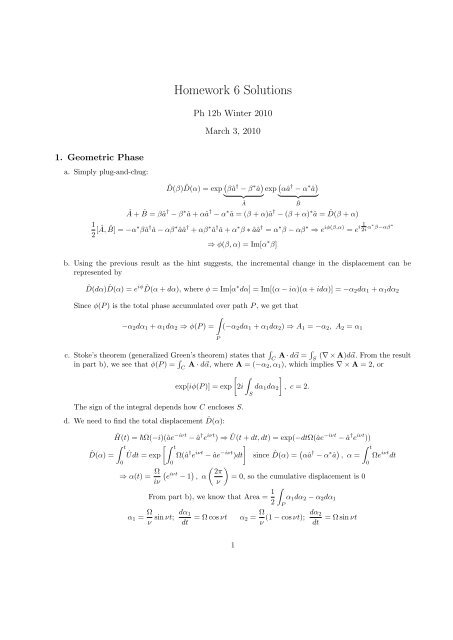
<strong>Homework</strong> 6 <strong>Solutions</strong><br />
Ph 12b Winter 2010<br />
March 3, 2010<br />
1. Geometric Phase<br />
a. Simply plug-and-chug:<br />
ˆD(β) ˆD(α) = exp ( βâ † − β ∗ â )<br />
exp ( αâ † − α ∗ â )<br />
} {{ } } {{ }<br />
Â<br />
ˆB<br />
 + ˆB = βâ † − β ∗ â + αâ † − α ∗ â = (β + α)â † − (β + α) ∗ â = ˆD(β + α)<br />
1<br />
2 [Â, ˆB] = −α ∗ βâ † â − αβ ∗ ââ † + αβ ∗ â † â + α ∗ β ∗ ââ † = α ∗ β − αβ ∗ ⇒ e iϕ(β,α) = e i 1 2i α∗ β−αβ ∗<br />
⇒ ϕ(β, α) = Im[α ∗ β]<br />
b. Using the previous result as the hint suggests, the incremental change in the displacement can be<br />
represented by<br />
ˆD(dα) ˆD(α) = e iϕ ˆD(α + dα), where ϕ = Im[α ∗ dα] = Im[(α − iα)(α + idα)] = −α 2 dα 1 + α 1 dα 2<br />
Since ϕ(P ) is the total phase accumulated over path P , we get that<br />
∫<br />
−α 2 dα 1 + α 1 dα 2 ⇒ ϕ(P ) = (−α 2 dα 1 + α 1 dα 2 ) ⇒ A 1 = −α 2 , A 2 = α 1<br />
P<br />
c. Stoke’s theorem (generalized Green’s theorem) states that ∫ C A · d⃗α = ∫ (∇ × A)d⃗α. From the result<br />
S<br />
in part b), we see that ϕ(P ) = ∫ C A · d⃗α, where A = (−α 2, α 1 ), which implies ∇ × A = 2, or<br />
[ ∫ ]<br />
exp[iϕ(P )] = exp 2i dα 1 dα 2 , c = 2.<br />
S<br />
The sign of the integral depends how C encloses S.<br />
d. We need to find the total displacement ˆD(α):<br />
Ĥ(t) = Ω(−i)(âe −iνt − â † e iνt ) ⇒ Û(t + dt, dt) = exp(−dtΩ(âe−iνt − â † e iνt ))<br />
∫ t<br />
[∫ t<br />
]<br />
ˆD(α) = Ûdt = exp Ω(â † e iνt − âe −iνt )dt since ˆD(α) = ( αâ † − α ∗ â ) ∫ t<br />
, α = Ωe iνt dt<br />
0<br />
0<br />
0<br />
⇒ α(t) = Ω (<br />
e iνt − 1 ) ( ) 2π<br />
, α = 0, so the cumulative displacement is 0<br />
iν<br />
ν<br />
From part b), we know that Area = 1 ∫<br />
α 1 dα 2 − α 2 dα 1<br />
2<br />
α 1 = Ω ν sin νt; dα 1<br />
dt<br />
= Ω cos νt α 2 = Ω ν (1 − cos νt); dα 2<br />
dt<br />
P<br />
= Ω sin νt<br />
1
⇒ A = 1 2<br />
∫ 2π/ν<br />
0<br />
Ω<br />
ν sin νt · Ω sin νtdt − Ω Ω2<br />
(1 − cos νt) · Ω cos νtdt = π<br />
ν ν 2<br />
⇒ Geometric Phase: e i2πΩ2 /ν 2<br />
e. First evaluate σ 3 ⊗ I + I ⊗ σ 3 :<br />
⎧<br />
⎨ 0 |0⟩ ⊗ |1⟩, |1⟩ ⊗ |0⟩ and the rest<br />
σ 3 ⊗ I + I ⊗ σ 3 = 2 |0⟩ ⊗ |0⟩<br />
⎩<br />
−2 |1⟩ ⊗ |1⟩<br />
Applying the above to the two-qubit unitary operator ˆV is similar to what we got above for d). The area<br />
for these 3 possible conditions is 0 and 4πΩ 2 /ν 2 . Then the eigenvalues for ˆV<br />
(<br />
are e 8πΩ2 ν 2 , 1, 1, e 8πΩ2 ν 2) .<br />
If ν = 4Ω, the eigenvalues reduce to (i, 1, 1, i) and give time t = π/4Ω.<br />
2. Squeezing an Oscillator<br />
Note: all operators can commute with themselves (or powers thereof)!<br />
a. This is simple enough to prove as a general equality:<br />
(<br />
(e ϵ ˆB) ∑ ∞ † (ϵ<br />
=<br />
ˆB)<br />
) † n<br />
=<br />
n!<br />
n<br />
∞∑ (ϵ ˆB † ) n<br />
n<br />
n!<br />
=<br />
∞∑ (−ϵ ˆB) n<br />
n<br />
n!<br />
= e −ϵ ˆB ϵ<br />
= (e<br />
ˆB) −1<br />
and is thus unitary.<br />
b. Find the Taylor expansion around ϵ = 0 :<br />
( )<br />
Ĝ(ϵ) = e ϵ ˆB † ( ) ( ) ( )<br />
 e ϵ ˆB = e −ϵ ˆB  e ϵ ˆB ⇒ Ĝ(ϵ) = Ĝ(0) + ϵĜ′ (0) + · · ·<br />
= Â − ϵ ˆBe −ϵ ˆB Âe ϵ ˆB + ϵe −ϵ ˆB ϵ ˆB<br />
 ˆBe ∣ + · · · =  − ϵ ˆB + ϵ ˆB + · · · =  + ϵ[Â, ˆB]<br />
0<br />
c. Use the result from b) to speed up the process. Set ϵ = r/2 (ϵ/2), Â = â (â † ) and ˆB = â 2 − (â † ) 2 :<br />
Ŝ(ϵ) † âŜ(ϵ) = â + ϵ [â,<br />
â 2 − (â † ) 2] = â − ϵ [â,<br />
(â † ) 2] = â + ϵ 2<br />
2<br />
2 {↠[â, â † ] + [â, â † ]â † } = â − ϵa †<br />
Ŝ(ϵ) † â † Ŝ(ϵ) = â † + ϵ [↠, â 2 − (â † ) 2] = â † − ϵ [↠, â 2] = â † + ϵ 2<br />
2<br />
2 {â[↠, â] + [â † , â]â} = â † − ϵa<br />
d. Manipulate the operators such that above expansions can be used:<br />
Ŝ(ϵ) † ˆξŜ(ϵ) = Ŝ(ϵ)† 1 √<br />
2<br />
(â + â † )Ŝ(ϵ) = 1 √<br />
2 {Ŝ(ϵ)† âŜ(ϵ) + Ŝ(ϵ)† â † Ŝ(ϵ)} = 1 √<br />
2<br />
{(â + â † ) − ϵ(â + â † )}<br />
Ŝ(ϵ) † ˆp ξ Ŝ(ϵ) =<br />
= (1 − ϵ)ˆξ<br />
−i † −i<br />
Ŝ(ϵ)† √ (â − â )Ŝ(ϵ) = √<br />
2 2 {Ŝ(ϵ)† âŜ(ϵ) − Ŝ(ϵ)† â † Ŝ(ϵ)} = √ −i {(â − â † ) + ϵ(â − â † )}<br />
2<br />
= (1 + ϵ)ˆp ξ<br />
e. Subsituting r for ϵ and using the limit definition of e,<br />
lim<br />
(1 = − r ) N<br />
ˆξ = e<br />
−r ˆξ and lim<br />
(1<br />
N→∞ N<br />
= + r ) N<br />
ˆpξ = e r ˆp ξ<br />
N→∞ N<br />
2
f. Subsitute:<br />
⟨r|ˆξ|r⟩ = ⟨0|Ŝ(r)† ˆξŜ(r)|0⟩ = ⟨0|e −r ˆξ|0⟩ = e −r ⟨0|ˆξ|0⟩ = 0 by definition<br />
With this, we can calculate the variances:<br />
⟨r|ˆξ 2 |r⟩ = e −2r ⟨0| ˆξ 2 |0⟩ = e−2r<br />
2 ⟨0|â↠+ â † â|0⟩ = 1 2 e−2r<br />
⟨r|ˆp ξ |r⟩ = e r ⟨0|ˆp ξ |0⟩ = 0<br />
⟨r|ˆp 2 ξ|r⟩ = e2r<br />
2 ⟨0|â↠+ â † â|0⟩ = 1 2 e2r<br />
(∆ˆξ) r = 1 √<br />
2<br />
e −r and (∆ˆp ξ ) r = 1 √<br />
2<br />
e r<br />
which implies that the minimum uncertainty in this state has been “squeezed” to ∆ˆξ∆ˆp ξ = 1/2.<br />
3. Anharmonic Oscillator<br />
a. Rewrite the energy expression to express the peturbative term:<br />
E ′ n − E n = kω⟨n|ξ 4 |n⟩ = 1 4 kω⟨n|(â + ↠) 4 |n⟩<br />
In the expansion for (â + â † ) 4 , only terms with two raising and lowering operators would contribute;<br />
all others would shift |n⟩ into an orthogonal state. Thus we get<br />
(â + â † ) 4 =  = ââ↠⠆ + ââ † ââ † + ââ † â † â + â † âââ † + â † ââ † â + â † â † ââ<br />
â|n⟩ = √ n + 1|n + 1⟩ â † |n⟩ = √ n|n − 1⟩ ââ † |n⟩ = (n + 1)|n⟩ â † â|n⟩ = n|n⟩<br />
1<br />
4 kω⟨n|Â|n⟩ = 1 4 kω{(n + 1)(n + 2) + (n + 1)2 + n(n + 1) + n(n + 1) + n 2 + n(n − 1)}<br />
b. Evaluate the above expression:<br />
⇒ kω⟨n|ξ 4 |n⟩ = 1 4 kω(6n2 + 6n + 3)<br />
E 10 ′ = E 1 ′ − E 0 ′ = E 1 + 15<br />
4 kω − E 0 − 3 12<br />
kω = ω +<br />
4 4 kω<br />
E 21 ′ = E 2 ′ − E 1 ′ = E 2 + 39<br />
4 kω − E 1 − 15<br />
24<br />
kω = ω +<br />
4 4 kω<br />
∆(k) = E′ 21 − E 10<br />
′ 3kω<br />
E 10<br />
′ =<br />
ω + 3kω<br />
This gives 3k after Taylor expanding with regards to k around 0 and choosing the first term.<br />
3