Physics 205a, Problem Set 5 Solutions
Physics 205a, Problem Set 5 Solutions
Physics 205a, Problem Set 5 Solutions

You also want an ePaper? Increase the reach of your titles
YUMPU automatically turns print PDFs into web optimized ePapers that Google loves.
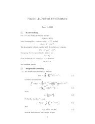
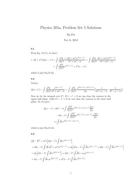
<strong>Physics</strong> <strong>205a</strong>, <strong>Problem</strong> <strong>Set</strong> 5 <strong>Solutions</strong><br />
Du Pei<br />
Nov 6, 2012<br />
8.1<br />
From Eq. (8.11), we have:<br />
∫<br />
(−∂x 2 + m 2 )∆(x − x ′ ) =<br />
which is just Eq.(8.12).<br />
8.2<br />
∫<br />
=<br />
d 4 k (−∂x 2 + m 2 )e ik(x−x′ )<br />
∫<br />
(2π) 4 k 2 + m 2 =<br />
− iϵ<br />
d 4 k<br />
(2π) 4 eik(x−x′) = δ 4 (x − x ′ ),<br />
d 4 k (k 2 + m 2 )e ik(x−x′ )<br />
(2π) 4 k 2 + m 2 − iϵ<br />
Notice:<br />
∫<br />
∆(x−x ′ ) =<br />
d 4 k e ik(x−x′ )<br />
∫<br />
(2π) 4 k 2 + m 2 − iϵ =<br />
d 4 k e i⃗ k(⃗x−⃗x ′ )−ik 0 (t−t ′ ) (<br />
(2π) 4 2ω<br />
1<br />
k 0 + ω − iϵ − 1<br />
k 0 − ω − iϵ<br />
)<br />
.<br />
Now we do the integral over k 0 . If t − t ′ < 0 we can close the contour in the<br />
upper half plane, while if t − t ′ > 0 we can close the contour in the lower half<br />
plane. So we have:<br />
which is just Eq.(8.13).<br />
∫<br />
∆(x − x ′ ) =θ(t ′ d 3⃗ k<br />
− t)<br />
(2π) 4 ei⃗ k(⃗x−⃗x ′ )+iω(t−t ′ ) 2πi<br />
2ω<br />
∫<br />
− θ(t − t ′ d 3⃗ k<br />
)<br />
(2π) 4 ei⃗ k(⃗x−⃗x ′ )−iω(t−t ′ ) −2πi<br />
2ω<br />
∫<br />
=i ˜dk e i⃗ k(⃗x−⃗x ′ )−iω|t−t ′| ,<br />
8.3<br />
[ ∫<br />
(∂t 2 − ∇ 2 + m 2 ) iθ(t − t ′ ) ˜dk ]<br />
e ik(x−x′ )<br />
∫<br />
∫<br />
∫<br />
= iθ(t − t ′ ) ˜dk ( ⃗ k 2 + m 2 )e ik(x−x′) + ∂ 0<br />
[iδ(t − t ′ ) ˜dk e ik(x−x′) + iθ(t − t ′ )<br />
∫<br />
= ∂ 0<br />
[iδ(t − t ′ ) ˜dk ] ∫<br />
e i⃗ k(⃗x−⃗x ′ )<br />
+ iδ(t − t ′ ) ˜dk (−iω)e ik(x−x′ )<br />
∫<br />
∫<br />
= δ(t − t ′ ) ˜dk ωe i⃗ k(⃗x−⃗x ′) + iδ ′ (t − t ′ ) ˜dk e i⃗ k(⃗x−⃗x ′) .<br />
˜dk e ik(x−x′ ) ]<br />
1
Similarly,<br />
[ ∫<br />
(∂t 2 − ∇ 2 + m 2 ) iθ( ′ t − t) ˜dk ]<br />
e −ik(x−x′ )<br />
∫<br />
∫<br />
= δ(t − t ′ ) ˜dk ωe i⃗ k(⃗x−⃗x ′) − iδ ′ (t − t ′ ) ˜dk e i⃗ k(⃗x−⃗x ′) .<br />
Combining those results we have:<br />
∫<br />
(∂x+m 2 2 )∆(x−x ′ ) = δ(t−t ′ )<br />
8.4<br />
∫<br />
˜dk 2ωe i⃗ k(⃗x−⃗x ′) = δ(t−t ′ )<br />
Bringing Eq. (3.19) into the time-ordered product gives:<br />
d 3 k<br />
(2π) 3 ei⃗ k(⃗x−⃗x ′) = δ 4 (x−x ′ ).<br />
⟨0|Tϕ(x 1 )ϕ(x 2 )|0⟩<br />
∫<br />
)<br />
= ˜dk 1˜dk2 ⟨0|T<br />
(a ⃗k1 e i⃗ k 1 ⃗x 1 −iω 1 t 1<br />
+ a † ⃗<br />
e −i⃗ k 1 ⃗x 1 +iω 1 t 1<br />
)(a ⃗k2 e i⃗ k 2 ⃗x 2 −iω 2 t 2<br />
+ a † k1 ⃗<br />
e −i⃗ k 2 ⃗x 2 +iω 2 t 2<br />
|0⟩<br />
k2<br />
∫<br />
]<br />
= ˜dk<br />
[θ(t 1 − t 2 )e −i⃗ k 1 ⃗x 1 +iω 1 t 1<br />
e −i⃗ k 2 ⃗x 2 +iω 2 t 2<br />
+ θ(t 2 − t 1 )e −i⃗ k 1 ⃗x 1 +iω 1 t 1<br />
e i⃗ k 2 ⃗x 2 −iω 2 t 2<br />
∫<br />
∫<br />
= θ(t 2 − t 1 ) ˜dke ik(x 2−x 1 ) + θ(t 1 − t 2 ) ˜dke −ik(x 2−x 1 ) = 1 i ∆(x 2 − x 1 ).<br />
8.5<br />
For x 0 > y 0 , we can close the contour in the lower k 0 plane. The integral will<br />
only vanish if both poles are above the real axis. So in the denominator, we<br />
should have −(k 0 − iϵ) 2 + m 2 + ⃗ k 2 = k 2 + m 2 + iϵk 0 . Then we have for the<br />
retarded potential:<br />
∫<br />
∆ ret (x − y) =<br />
d 4 k e ik(x−y)<br />
(2π) 4 k 2 + m 2 + iϵk 0 .<br />
And similarly, for x 0 < y 0 we can close the contour in the upper k 0 plane, so<br />
the pole prescription that will work for the advanced potential is:<br />
∫<br />
∆ adv (x − y) =<br />
d 4 k e ik(x−y)<br />
(2π) 4 k 2 + m 2 − iϵk 0 .<br />
2