Ph219/CS219 Problem Set 3

Ph219/CS219 Problem Set 3
Solutions by Hui Khoon Ng
December 3, 2006
(KSV: Kitaev, Shen, Vyalyi, Classical and Quantum Computation)
3.1 The O(...) notation
We can do this problem easily just by knowing the following hierarchy:
s ≤ (log n) p ≤ n q ≤ r n
(S1)
for any constants s, p, q, r greater than 1, and the log can be to any base. The “≤” sign stands
for the O-relation.
Let us transform some of the functions in question:
• n log n = cn ln n (more precisely, n log a n = n ln n ). Using the “=” sign for the bidirectional
ln a
O-relation, we may write “n log n = n ln n”. One must be careful, though – see the next
item;
• (log 2 n) n = (1/ ln 2) n (ln n) n . Note that 1/ ln 2 > 1, hence (log 2 n) n > (ln n) n in the
O-relation sense;
• (ln n) n = e (ln ln n)n . This function grows faster than a n = e (ln a)n for any constant a. Indeed
f(n) ≤ O(g(n)) implies that e f(n) ≤ O ( e g(n)) . Proof:
f ≤ O(g) ⇒ f(n) ≤ cg(n)
⇒ e f(n) ≤ e c e g(n)
⇒ e f(n) ≤ (constant)e g(n) ;
∀n ≥ n 0 , some c
• n ln n = e (ln n)2 . This function grows faster than any constant power of n, yet not as fast
as an exponential function.
• n! ≈ √ 2πn ( )
n n
using Stirling’s formula;
e
• ( )
2n
n =
(2n)!
≈ 4n
(n!) 2 √ πn
;
• ln(n!) ≈ ln √ 2π + 1 2 ln n + n ln n ≈ n ln n; 1

• ln ( )
2n
√
n ≈ − ln π −
1
ln n + n ln 4 ≈ n ln 4.
2
Putting all these together, the ordering of the functions is
( )
( )
2n 2n
n = ln < n log n = ln(n!) < n ln n < 2 n < < (ln n) n < (log
n n 2 n) n < n! .
3.2 Programming a Turing Machine
(a) We
∑
are given the n-digit binary number u written backwards on the tape as x 0 x 1 x 2 . . . x n−1 =
n−1
k=0 2k x k , x k ∈ {0, 1}, and we want to increment it by 1. To do this, we start with the
cell on the left end of the tape containing x 0 , if it is 1, change it to 0, and move right by
one step; if x 1 is 1, change it to 0 and move right by one step; etc. We repeat this until we
see the first 0 or a blank symbol (marking the end of the input) on the tape, we change
that to 1 and stop. This procedure is implemented by the rules below, with external
alphabet given as A = {0, 1}, internal alphabet S = A ∪ { }, and Turing machine (TM)
states Q = {α, β}, where α is the initial state of the TM and β will be used as the stop
state. Recall the notation: (q, s) −→ (q ′ , t, step) means the current TM state is q, the
symbol in the current cell (where the head is) is s, and the transition is to a new state
q ′ , the head writes symbol t in current cell, and then moves by step. The rules are as
follows:
(α, 0) −→ (β, 1, 0)
(α, 1) −→ (α, 0, +1)
(α, ) −→ (β, 1, 0).
The TM stops when it goes into the β state. Note that this TM increments the input by
1 even if the input tape is blank (i.e. u is 0-bit number).
(b) We want to duplicate the input binary string bit by bit, i.e. we want to convert x 0 x 1 . . . x n−1
into x 0 x 0 x 1 x 1 . . . x n−1 x n−1 . One way to do this is to clear the cell immediately to the right
of the symbol we want to duplicate by shifting all symbols to the right by one cell. The
external alphabet is given as A = {0, 1}, we will use internal alphabet S = A ⋃ { }, and
the state set Q = {α, r 0 , r 1 , l 0 , l 1 , w}. The procedure is as follows (s, t ∈ {0, 1}):
Step 1: Pick up the symbol in the current cell which we want to duplicate, put a blank
symbol in its place to mark the position, and move to the right. Swap the symbol we
picked before with the one on the tape and move to the right again. Repeat until we see
the end of the input.
(α, s) −→ (r s , , +1)
(r s , t) −→ (r t , s, +1)
(r s , ) −→ (l s , s, −1)
2

Step 2: Move left until we find a blank symbol — the mark we left on Step 1. Put a copy
of the symbol we saw last and make two step rightwards. Then return to Step 1.
(l s , t) −→ (l t , t, −1)
(l s , ) −→ (w, s, +1)
(w, s) −→ (α, s, +1)
Does this TM stop? After it is done duplicating the input, it will be in state α, but its
current cell symbol will be , for which there is no rule defined, so machine stops.
(c) The idea is to use a fixed length code based on the symbols in A = {0, 1} to represent the
internal alphabet S ⊃ A. Let us try to understand the details of how this works through
an example. Suppose we have a TM that uses the internal alphabet S = A ⋃ {2, }.
Instead of using the additional symbol 2, we can have another TM that carries out the
same program with the internal alphabet S = A ⋃ { } by using the following 2-bit code
to represent all symbols of S:
0 → 00, 1 → 11, 2 → 01, → 10.
We have chosen not to use the blank symbol in the encoding but rather reserve it for
other purposes (see below).
When the input tape is given to the TM, with symbols from the external alphabet
A = {0, 1}, the TM first does an encoding of the input, i.e., duplicating all input symbols
according to the code so that the input x 0 x 1 . . . x n−1 becomes x 0 x 0 x 1 x 1 . . . x n−1 x n−1 .
Notice that this is exactly part (b) of this problem, the solution of which used only the
internal alphabet consisting of 0, 1, and . Once the TM is done encoding the input,
it performs the actual computation using the encoded input and the encoded internal
symbols 2, . Note that the fixed length code allows the TM to recognize the correct
internal symbol by reading the cells on the tape two at a time (one after another). When
it is done, the TM returns to the left end of the tape and decodes the output back into
0’s and 1’s, i.e. 00 → 0 and 11 → 1.
(There is a technical problem here: the definition given in class or in KSV does not allow
a TM to see the left end of the tape before crashing into it. To cope with this difficulty,
we may insert a blank symbol at the left end of the tape as a cushion. Furthermore, we
have to avoid using blanks in our computation, which is the reason for the rule → 10.
If the machine must move beyond the original encoded region, it will recognize a pair
of blanks as an encoded blank, replacing it by the suitable combination of 0’s and 1’s.
This way, 0’s and 1’s will always occupy a contiguous region, making it easy to locate the
cushion symbol.)
A similar procedure can be used for a TM with S consisting of a larger set of symbols,
just by using a longer code, with 0 represented as 00 . . . 0, 1 as 11 . . . 1, and other symbols
represented by other codewords of the same length. The encoding phase can be carried
out in a similar fashion as above, using only the internal symbols 0,1 and .
3

3.3 The Threshold Function
(a) There are a few ways of doing this part, one of which is to think of this as sorting the
input string of x 1 , . . . , x n into a string with all the 1’s in front of all the 0’s. Another way
of doing this is to start with a string of n 0’s, and shift 1’s rightwards when the input is
a 1. The circuit that does this is shown in Fig. 1, where q 0 = 00 . . . 0 is a string of n 0’s,
and q k = q k,1 q k,2 . . . q k,n is the encoding of y k = ∑ k
j=1 x j as 1 } .{{ . . 1}
0 } .{{ . . 0}
. In particular, q n
y k n−y k
is the string representing ∑ n
j=1 x j as required. The k-th bit of q n gives the value of the
THRESHOLD function.
Figure 1: The circuit for Problem 3 (a).
x 1
q 0
x 2
q 1
q k−1
:
q k−1,1
q k−1,2
q k−1,3
q k−1,n
q 2
q n−1
x k
q k
:
x n
q
n
q k,1
q k,2
q k,3
q k,n
Each box in this circuit is of size O(n) and constant depth, and we have n boxes in
sequence. Therefore, the total circuit size is O(n 2 ) and depth O(n).
(b) Recall from class that there exists a circuit of size O(m) and depth O(1) that converts
the sum of three m-digit numbers into a sum of two numbers, one of which is an m-digit
number and the other an (m + 1)-digit number. (If you want the details of the proof,
refer to the lemma in the solution of KSV problem 2.13.) Using this circuit twice, we can
convert a sum of four m-digit numbers into a sum of two (m + 1)-digit numbers. We are
going to use this in our algorithm described below.
Take n = 2 l for some integer l (if this is not true, append the input data with 0’s). Let
us construct a tree, with the n bits of input data x 1 , x 2 , . . . , x n as the leaves, and at each
node, we add the values of the two input leaves to the node. At the first level, we do
nothing, and just write x j +x j+1 at the node with input leaves x j and x j+1 . At the second
level, at each node, we convert the sum of four numbers (x j−2 + x j−1 ) + (x j + x j+1 ) to a
sum of two numbers using the constant depth circuit mentioned above. We end up with
a sum of two 2-bit numbers at each node. Repeat this procedure for every level of the
tree, each time converting the sum of four m-digit numbers at each node into a sum of
4

two m + 1-digit numbers. We end up with two (log n)-digit numbers at the root of the
tree. This tree is shown in Figure 2.
Level 0:
Figure 2:
x1
x2
x 3 x 4
x 5 x 6
x 7 x 8
x n−1
x n
Level 1:
x 1 + x x +
2 3 x x +
4 5 x 6 x 7 + x x 8 n−1 + x n
Level 2:
(x 1+
x 2) +(x 3 + x 4 )
+
u 1 + u 2
(x 5 x 6 ) +(x 7 + x 8 )
u 3 + u 4
Level 3:
v 1 + v 2
Level
(log n):
z 1 + z 1
Let us figure out the circuit complexity of this tree. At level 1, we do nothing, so the
circuit size and depth are both constant. At level 2, we have n/2 nodes, at each of which,
we convert four 1-bit numbers into two 2-bit numbers, so the size is n/2 · O(2), and depth
is constant. At level k, we have n/2 k−1 nodes, at each of which, we convert four (k−1)-bit
numbers into two k-bit numbers, so the size is n/2 k−1 · O(k) and depth is still constant.
We have log n levels in total, hence,
size =
log n
∑
k=1
(
log n−1
nO(k) ∑
= O n
2 k−1 k=0
) (
k
≤ O n
2 k
∞∑
k=0
)
k
= O(n),
2 k
since the series ∑ ∞ k
k=0
converges. The depth is O(log n).
2 k
At the root of the tree, we have two (log n)-digit numbers denoted as z 1 and z 2 . We want
a binary output at the end of the procedure, so we still have to do the actual binary sum
of z 1 and z 2 , which can be done with the parallel addition circuit with depth O(log log n)
and size O(log n).
Altogether then, the circuit complexity is:
size = O(n) + O(log n) = O(n),
depth = O(log n) + O(log log n) = O(log n).
— better than the problem asks for!
5

∑
To get the value of the THRESHOLD function, we need to compute the difference
n
∑j=1 x j − k and compare the result with 0. To do this, we write the difference as
n
j=1 x j + (−k) and use the complementary code to represent −k in binary. (Google
”two’s complement” if you are not familiar with this. Briefly, to represent negative numbers
for m-digit numbers, we use an (m + 1)-digit binary string, with the first bit being
the sign bit, i.e. it is 0 if the number is non-negative, 1 if negative. To read the complementary
code when the sign bit is 1, we flip all the bits in the (m + 1)-bit string and add
1. The number represented is then the negative of the resulting string.) Then, do the
binary sum of ∑ n
j=1 x j and −k, which we can do with size O(log n) and depth O(log log n)
since both are O(log n)-digit numbers, and the value of the THRESHOLD function is the
value of the sign bit of the result.
3.4 Measurement Decoding
We are given n readings s 0 , s 1 , . . . , s n−1 ∈ {0, 1, . . . , 7} from n meters differing in rotation speeds
by a factor of 2, with the s 0 meter being the slowest. We are promised that these ( readings ) are
consistent estimates of a number x between 0 and 1 such that 2 j sj −1
x(mod 1) ∈ , s j+1
. Let
8 8
us define β j := s j
, then, 8
∣ ∣ ∣(2 j x − β j ) mod 1 1 < for j = 0, 1, . . . , n − 1.
8
The problem is to combine the overlapping information from the n readings to get an estimate
y of x such that |(x − y) mod 1 | < 2 −(n+2) .
First, a simple fact that we will use: suppose |(2a − .b 1 b 2 b 3 . . .) mod 1 | < δ < 1 , then exactly
2
one of the following is true:
either ∣ ( a − .0b 1 b 2 . . . ) ∣ < δ/2
mod 1
or ∣ ( a − .1b 1 b 2 . . . ) ∣
mod 1 < δ/2.
(S2)
For each j, let us write β j := .b j1 b j2 b j3 (note that we only need three digits since β j = integer/8).
Given |(2 j x − β j ) mod 1 | < 1/8, using (S2), we also know that either |(2 j−1 x − .0b j1 b j2 b j3 ) mod 1 | <
1/16 or |(2 j−1 x − .1b j1 b j2 b j3 ) mod 1 | < 1/16. Repeating this procedure, we eventually get 2 j possible
regions, each of length 2 −(j+2) , in which x can lie which are consistent with the given value
of β j . Since the data are consistent, there will be a finite region contained in the intersection
of the sets of regions from the different j values. This region is of length 2 −(n+1) and contains
x. If we take y as the midpoint of this region, then |(x − y) mod 1 | < 2 −(n+2) .
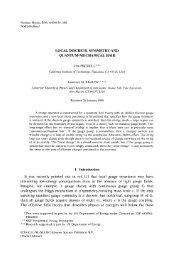
Let us look at a specific example. Consider x = .011101, which we know just to check our
results. Take n = 3. Then, we can have the data s 0 = 4, s 1 = 7, s 2 = 7. We can check that this
6

Figure 3: s 0 meter, pointer indicates value of x.
7
0
1
6
2
5
4
3
¡¡¡
¢¡¢¡¢¡¢¡¢
¡¡¡
¢¡¢¡¢¡¢¡¢
¡¡¡
¢¡¢¡¢¡¢¡¢
¡¡¡
¢¡¢¡¢¡¢¡¢
set of data satisfies the required conditions:
(
∣ x − s )
0
∣ = ∣ ∣
∣ ∣∣∣ .011101 − .100 = − 1 8 mod 1
2 + 1 4 + 1 8 + 1 16 + 1
64∣ = 3 64 < 1 8 ,
(
∣ 2x − s )
1
∣ = ∣ ∣ .11101 − .111 1 =
8 mod 1
64 < 1 8 ,
(
∣ 2 2 x − s )
2
∣ = ∣ ∣
∣ ∣∣∣ .1101 − .111 = − 1 8 mod 1
8 + 1
16∣ = 1
16 < 1 8 .
Using (S2) repeatedly, from s 2 , we get four possible regions in which x can lie, each of
length 1/16 (see Fig. 3), from s 1 , two regions, each of length 1/8, and from s 0 , one region of
length 1/4. The shaded region (of length 1/16 as constrained by the region coming from s 2 )
corresponds to the overlap between all the different s j values. As can be seen from the diagram,
x indeed lies in this region, and we get the desired precision if we take y as the midpoint of the
shaded region.
(a) How do we get the correct value of y with circuit size O(n)? The problem is, of course, that
there are exponentially many regions. Fortunately, we do not need to list all of them. 1 Let
1 A subtle point to note is that there is more than one possible set of values for {s j } that is consistent with a
given x. For instance, in the example above, s 0 could have been 3 instead of 4, and we would still get the same
shaded region. This causes the following seemingly plausible strategy to fail to give the correct y: write each
β j in the binary fraction representation β j = .b j1 b j2 b j3 and take y = .b 01 b 11 b 21 . . . b n−2,1 b n−1,1 b n−1,2 b n−1,3 , i.e.
start with β n−1 = .b n−1,1 b n−1,2 b n−1,3 , and prepend with the first digit of β n−2 , β n−3 , . . . , β 0 . In our example,
if the data is given as s 0 = 3, s 1 = 7, s 2 = 7, this strategy gives y = .01111 which is within 1/16 of the value of
x. However, if the data is given as s 0 = 4, s 1 = 7, s 2 = 7, we get y = .11111, which is not within the desired
precision. It is easy to see that this strategy only works if we are given s j values that are the nearest tick marks
counterclockwise from the pointer for 2 j x on the respective meters.
7

us go back to our original argument. The inequalities |(2 j−1 x − .0b j1 b j2 b j3 ) mod 1 | < 1/16
and |(2 j−1 x − .1b j1 b j2 b j3 ) mod 1 | < 1/16 define two arcs of length 1/8 on opposite sides
of the circle. Only one of the arcs can overlap with the region defined by the inequality
|(2 j−1 x−β j−1 ) mod 1 | < 1/8 because the length of this region (1/4) is smaller than the gaps
between the arcs (3/8). Therefore, we can select the right arc before further multiplying
the number of choices. This observation suggest the following algorithm, in which we
work out the bits of y right to left.
Let us start with the binary representation of β n−1 := .y n y n+1 y n+2 . Now, sequentially
pick y k , k = n − 1, n − 2, . . . , 1 such that
{ ( )
0 if .0yk+1 − β k−1
y k =
1 if ( ) ∈ { − 2, − 1, 0, mod 1 8 8 8 8} 1 ,
.1y k+1 − β k−1 ∈ { − 2 , − 1 , 0 , } 1 (S3)
mod 1 8 8 8 8 .
(Note that exactly one of these two conditions holds.) Then, take y = .y 1 y 2 . . . y n y n+1 y n+2 .
We need to check that y found this way gives the required precision for x, i.e., |(x − y) mod 1 | <
2 −(n+2) . We prove this using induction on the statement:
| ( .y k y k+1 . . . y n+2 − 2 k−1 x ) mod 1 | < δ k, where δ k = 2 −(n+3−k) . (S4)
Base case. If k = n then
∣ ( .y n y n+1 y n+2 − 2 n−1 x ) ∣
mod 1 = |(βn−1 − 2 n−1 x) mod 1 | < 2 −3 = δ n .
Induction step. Assume that equation (S4) is true for some k; we need to prove it for
˜k = k − 1. The inductive assumption implies that
∣ ( .uy k y k+1 . . . y n+2 − 2 k−2 x ) ∣
δ k
mod 1 <
2 = δ k−1
(S5)
for u = 0 or u = 1. We just need to check that (S3) gives the correct value for y k−1 , i.e.,
y k−1 = u. To see this, notice that
0 ≤ .uy k y k+1 . . . y n+2 − .uy k ≤
n+4−k
∑
j=3
2 −j = 1/4 − δ k−1 . (S6)
Using (S5) and (S6) together with the data consistency condition, |(2 k−2 x − β k−2 ) mod 1 | ≤
1/8, we get:
−δ k−1 − (1/4 − δ k−1 ) − 1/8 < (.uy k − β k−2 ) mod 1
< δ k−1 − 0 + 1/8.
Hence
as required.
(.uy k − β k−2 ) mod 1
∈ {−2/8, −1/8, 0, 1/8}
(S7)
8

Figure 4: O(n) circuit as a finite-state automaton.
β 0
✛
❄
F
(y 2 , y 3 )
✛
β n−3 β n−2
❄ ❄
(y n−1 , y n) (y n, y n+1 )
. . . ✛ ✛ ✛
F
F
❄
y 1
❄
y n−2
❄
y n−1
In this algorithm, y k depends only on β k and y k+1 . Proving the correctness by induction is
somewhat tricky, though. The proof may be easier to carry out if we replace condition (S3)
by, say, this inequality:
∣ ( )
.y k y k+1 y k+2 1 − β k−1
∣ < 1/4.
(S8)
mod 1
In this case, y k depends on β k , y k+1 , and y k+2 . However, the overall structure of the
algorithm remains the same. It can be viewed as a finite-state automaton F : (β, q) ↦→
(y, q) (where β ∈ {0, 1}, y ∈ {0, 1}, and q = (y ′ , y ′′ ) ∈ {0, 1} 2 denotes the state of the
automaton) defined as:
F (β k−1 , (y k+1 , y k+2 )) = (y k , (y k , y k+1 ))
with y k given by (S8). This is represented schematically in Fig. 4. The initial state of
the automaton is computed from β n−1 (which can be done with a constant size circuit).
Notice that F is computable by a fixed size circuit, but we need to repeat it n times in
sequence, so the circuit complexity is given by
size = O(n)
depth = O(n).
(b) From part (a), we know that our algorithm can be viewed as a finite-state automaton
operating n times in sequence. This point of view makes it very easy to see how to
parallelize the circuit, just by analogy with the parallelization of addition discussed in
class. Recall that in parallelizing addition, we compute all the carry-bits with depth
O(log n) by first computing the composition of functions given the input in the form of a
tree of depth O(log n). Here, the automaton state q k := (y k+1 , y k+2 ) plays the role of the
carry bit, which we need to compute the next value of y k . We carry out the exact same
procedure as in the case of parallelizing addition. We first compute all compositions of
the functions F βk : Q −→ Q in the form of a tree. This tree is of depth O(log n), with
O(n) nodes, each node corresponding to a composition of two fixed size functions (and
hence computable by a circuit with constant size and depth). Hence this composition
process has circuit size O(n) and depth O(log n). Having gotten all these composition
functions, we need to compute q k ∀k. This can be done in O(log n) steps, just like in the
9

Figure 5: Computing q values for n=8.
q 7
q 3
q
q
1
5
q q q q 0 2 4 6
q q q q q q q q
0 1 2 3 4 5 6 7
case of computing the carry bits in the parallel addition algorithm (see Figure 5 for an
example for n = 8). Finally, we compute in parallel, all the y k values given the q k values.
Altogether then, the circuit complexity is:
size = O(n),
depth = O(log n).
Note that all finite-state automaton algorithms of the above form can be parallelized
in the same way to reduce the depth from O(n) to O(log n). For further reference, see
the solution to KSV problem 2.11 (for simplicity, you can take the parameter k in that
problem to be a constant).
10