Chapter 7 Quantum Error Correction
Chapter 7 Quantum Error Correction
Chapter 7 Quantum Error Correction

Create successful ePaper yourself
Turn your PDF publications into a flip-book with our unique Google optimized e-Paper software.
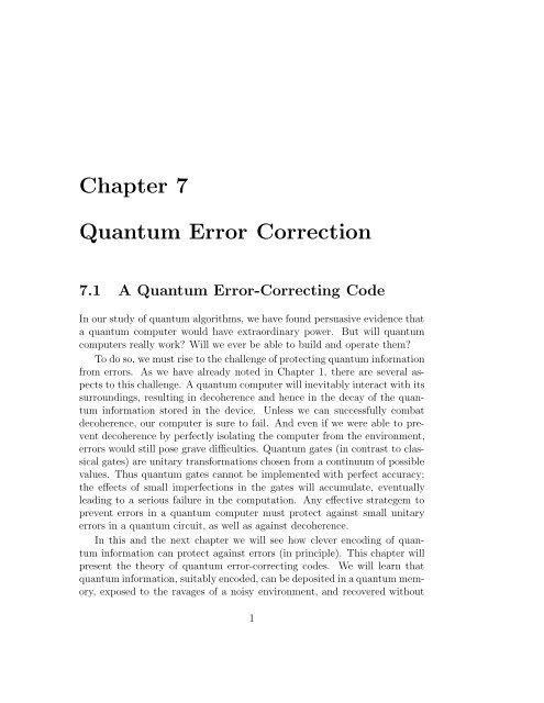
<strong>Chapter</strong> 7<br />
<strong>Quantum</strong> <strong>Error</strong> <strong>Correction</strong><br />
7.1 A <strong>Quantum</strong> <strong>Error</strong>-Correcting Code<br />
In our study of quantum algorithms, we have found persuasive evidence that<br />
a quantum computer would have extraordinary power. But will quantum<br />
computers really work? Will we ever be able to build and operate them?<br />
To do so, we must rise to the challenge of protecting quantum information<br />
from errors. As we have already noted in <strong>Chapter</strong> 1, there are several aspects<br />
to this challenge. A quantum computer will inevitably interact with its<br />
surroundings, resulting in decoherence and hence in the decay of the quantum<br />
information stored in the device. Unless we can successfully combat<br />
decoherence, our computer is sure to fail. And even if we were able to prevent<br />
decoherence by perfectly isolating the computer from the environment,<br />
errors would still pose grave difficulties. <strong>Quantum</strong> gates (in contrast to classical<br />
gates) are unitary transformations chosen from a continuum of possible<br />
values. Thus quantum gates cannot be implemented with perfect accuracy;<br />
the effects of small imperfections in the gates will accumulate, eventually<br />
leading to a serious failure in the computation. Any effective strategem to<br />
prevent errors in a quantum computer must protect against small unitary<br />
errors in a quantum circuit, as well as against decoherence.<br />
In this and the next chapter we will see how clever encoding of quantum<br />
information can protect against errors (in principle). This chapter will<br />
present the theory of quantum error-correcting codes. We will learn that<br />
quantum information, suitably encoded, can be deposited in a quantum memory,<br />
exposed to the ravages of a noisy environment, and recovered without<br />
1
2 CHAPTER 7. QUANTUM ERROR CORRECTION<br />
damage (if the noise is not too severe). Then in <strong>Chapter</strong> 8, we will extend the<br />
theory in two important ways. We will see that the recovery procedure can<br />
work effectively even if occasional errors occur during recovery. And we will<br />
learn how to process encoded information, so that a quantum computation<br />
can be executed successfully despite the debilitating effects of decoherence<br />
and faulty quantum gates.<br />
A quantum error-correcting code (QECC) can be viewed as a mapping<br />
of k qubits (a Hilbert space of dimension 2 k ) into n qubits (a Hilbert space<br />
of dimension 2 n ), where n > k. The k qubits are the “logical qubits” or<br />
“encoded qubits” that we wish to protect from error. The additional n − k<br />
qubits allow us to store the k logical qubits in a redundant fashion, so that<br />
the encoded information is not easily damaged.<br />
We can better understand the concept of a QECC by revisiting an example<br />
that was introduced in <strong>Chapter</strong> 1, Shor’s code with n = 9 and k = 1.<br />
We can characterize the code by specifying two basis states for the code subspace;<br />
we will refer to these basis states as |¯0〉, the “logical zero” and |¯1〉, the<br />
“logical one.” They are<br />
|¯0〉 = [ 1 √<br />
2<br />
(|000〉 + |111〉)] ⊗3 ,<br />
|¯1〉 = [ 1 √<br />
2<br />
(|000〉 − |111〉)] ⊗3 ; (7.1)<br />
each basis state is a 3-qubit cat state, repeated three times. As you will<br />
recall from the discussion of cat states in <strong>Chapter</strong> 4, the two basis states<br />
can be distinguished by the 3-qubit observable σ (1)<br />
x ⊗ σ (2)<br />
x ⊗ σ (3)<br />
x (where<br />
σ (i)<br />
x denotes the Pauli matrix σ x acting on the ith qubit); we will use the<br />
notation X 1 X 2 X 3 for this operator. (There is an implicit I ⊗ I ⊗ · · · ⊗ I<br />
acting on the remaining qubits that is suppressed in this notation.) The<br />
states |¯0〉 and |¯1〉 are eigenstates of X 1 X 2 X 3 with eigenvalues +1 and −1<br />
respectively. But there is no way to distinguish |¯0〉 from |¯1〉 (to gather any<br />
information about the value of the logical qubit) by observing any one or two<br />
of the qubits in the block of nine. In this sense, the logical qubit is encoded<br />
nonlocally; it is written in the nature of the entanglement among the qubits<br />
in the block. This nonlocal property of the encoded information provides<br />
protection against noise, if we assume that the noise is local (that it acts<br />
independently, or nearly so, on the different qubits in the block).<br />
Suppose that an unknown quantum state has been prepared and encoded<br />
as a|¯0〉 + b|¯1〉. Now an error occurs; we are to diagnose the error and reverse
7.1. A QUANTUM ERROR-CORRECTING CODE 3<br />
it. How do we proceed? Let us suppose, to begin with, that a single bit flip<br />
occurs acting on one of the first three qubits. Then, as discussed in <strong>Chapter</strong><br />
1, the location of the bit flip can be determined by measuring the two-qubit<br />
operators<br />
Z 1 Z 2 , Z 2 Z 3 . (7.2)<br />
The logical basis states |¯0〉 and |¯1〉 are eigenstates of these operators with<br />
eigenvalue 1. But flipping any of the three qubits changes these eigenvalues.<br />
For example, if Z 1 Z 2 = −1 and Z 2 Z 3 = 1, then we infer that the first<br />
qubit has flipped relative to the other two. We may recover from the error<br />
by flipping that qubit back.<br />
It is crucial that our measurement to diagnose the bit flip is a collective<br />
measurement on two qubits at once — we learn the value of Z 1 Z 2 , but we<br />
must not find out about the separate values of Z 1 and Z 2 , for to do so<br />
would damage the encoded state. How can such a collective measurement<br />
be performed? In fact we can carry out collective measurements if we have<br />
a quantum computer that can execute controlled-NOT gates. We first introduce<br />
an additional “ancilla” qubit prepared in the state |0〉, then execute the<br />
quantum circuit<br />
– Figure –<br />
and finally measure the ancilla qubit. If the qubits 1 and 2 are in a state<br />
with Z 1 Z 2 = −1 (either |0〉 1 |1〉 2 or |1〉 1 |0〉 2 ), then the ancilla qubit will flip<br />
once and the measurement outcome will be |1〉. But if qubits 1 and 2 are<br />
in a state with Z 1 Z 2 = 1 (either |0〉 1 |0〉 2 or |1〉 1 |1〉 2 ), then the ancilla qubit<br />
will flip either twice or not at all, and the measurement outcome will be |0〉.<br />
Similarly, the two-qubit operators<br />
Z 4 Z 5 , Z 7 Z 8 ,<br />
Z 5 Z 6 , Z 8 Z 9 , (7.3)<br />
can be measured to diagnose bit flip errors in the other two clusters of three<br />
qubits.<br />
A three-qubit code would suffice to protect against a single bit flip. The<br />
reason the 3-qubit clusters are repeated three times is to protect against
4 CHAPTER 7. QUANTUM ERROR CORRECTION<br />
phase errors as well. Suppose now that a phase error<br />
|ψ〉 → Z|ψ〉 (7.4)<br />
occurs acting on one of the nine qubits. We can diagnose in which cluster<br />
the phase error occurred by measuring the two six-qubit observables<br />
X 1 X 2 X 3 X 4 X 5 X 6 ,<br />
X 4 X 5 X 6 X 7 X 8 X 9 . (7.5)<br />
The logical basis states |¯0〉 and |¯1〉 are both eigenstates with eigenvalue one<br />
of these observables. A phase error acting on any one of the qubits in a<br />
particular cluster will change the value of XXX in that cluster relative to<br />
the other two; the location of the change can be identified by measuring the<br />
observables in eq. (7.5). Once the affected cluster is identified, we can reverse<br />
the error by applying Z to one of the qubits in that cluster.<br />
How do we measure the six-qubit observable X 1 X 2 X 3 X 4 X 5 X 6 ? Notice<br />
that if its control qubit is initially in the state √ 1<br />
2<br />
(|0〉 + |1〉), and its target is<br />
an eigenstate of X (that is, NOT) then a controlled-NOT acts according to<br />
CNOT :<br />
1<br />
√<br />
2<br />
(|0〉 + |1〉) ⊗ |x〉 → 1 √<br />
2<br />
(|0〉 + (−1) x |1〉) ⊗ |x〉;<br />
(7.6)<br />
it acts trivially if the target is the X = 1 (x = 0) state, and it flips the<br />
control if the target is the X = −1 (x = 1) state. To measure a product of<br />
X’s, then, we execute the circuit<br />
– Figure –<br />
and then measure the ancilla in the 1 √<br />
2<br />
(|0〉 ± |1〉) basis.<br />
We see that a single error acting on any one of the nine qubits in the block<br />
will cause no irrevocable damage. But if two bit flips occur in a single cluster<br />
of three qubits, then the encoded information will be damaged. For example,<br />
if the first two qubits in a cluster both flip, we will misdiagnose the error and<br />
attempt to recover by flipping the third. In all, the errors, together with our
7.2. CRITERIA FOR QUANTUM ERROR CORRECTION 5<br />
mistaken recovery attempt, apply the operator X 1 X 2 X 3 to the code block.<br />
Since |¯0〉 and |¯1〉 are eigenstates of X 1 X 2 X 3 with distinct eigenvalues, the<br />
effect of two bit flips in a single cluster is a phase error in the encoded qubit:<br />
X 1 X 2 X 3 : a|¯0〉 + b|¯1〉 → a|¯0〉 − b|¯1〉 . (7.7)<br />
The encoded information will also be damaged if phase errors occur in two<br />
different clusters. Then we will introduce a phase error into the third cluster<br />
in our misguided attempt at recovery, so that altogether Z 1 Z 4 Z 7 will have<br />
been applied, which flips the encoded qubit:<br />
Z 1 Z 4 Z 7 : a|¯0〉 + b|¯1〉 → a|¯1〉 + b|¯0〉 . (7.8)<br />
If the likelihood of an error is small enough, and if the errors acting on<br />
distinct qubits are not strongly correlated, then using the nine-qubit code<br />
will allow us to preserve our unknown qubit more reliably than if we had not<br />
bothered to encode it at all. Suppose, for example, that the environment<br />
acts on each of the nine qubits, independently subjecting it to the depolarizing<br />
channel described in <strong>Chapter</strong> 3, with error probability p. Then a bit<br />
flip occurs with probability 2 p, and a phase flip with probability 2 p. (The<br />
3 3<br />
probability that both occur is 1 p). We can see that the probability of a phase<br />
3<br />
error affecting the logical qubit is bounded above by 4p 2 , and the probability<br />
of a bit flip error is bounded above by 12p 2 . The total error probability is no<br />
worse than 16p 2 ; this is an improvement over the error probability p for an<br />
unprotected qubit, provided that p < 1/16.<br />
Of course, in this analysis we have implicitly assumed that encoding,<br />
decoding, error syndrome measurement, and recovery are all performed flawlessly.<br />
In <strong>Chapter</strong> 8 we will examine the more realistic case in which errors<br />
occur during these operations.<br />
7.2 Criteria for <strong>Quantum</strong> <strong>Error</strong> <strong>Correction</strong><br />
In our discussion of error recovery using the nine-qubit code, we have assumed<br />
that each qubit undergoes either a bit-flip error or a phase-flip error (or both).<br />
This is not a realistic model for the errors, and we must understand how to<br />
implement quantum error correction under more general conditions.<br />
To begin with, consider a single qubit, initially in a pure state, that interacts<br />
with its environment in an arbitrary manner. We know from <strong>Chapter</strong>
6 CHAPTER 7. QUANTUM ERROR CORRECTION<br />
3 that there is no loss or generality (we may still represent the most general<br />
superoperator acting on our qubit) if we assume that the initial state<br />
of the environment is a pure state, which we will denote as |0〉 E . Then the<br />
evolution of the qubit and its environment can be described by a unitary<br />
transformation<br />
U : |0〉 ⊗ |0〉 E → |0〉 ⊗ |e 00 〉 E + |1〉 ⊗ |e 01 〉 E ,<br />
|1〉 ⊗ |0〉 E → |0〉 ⊗ |e 10 〉 E + |1〉 ⊗ |e 11 〉 E ; (7.9)<br />
here the four |e ij 〉 E are states of the environment that need not be normalized<br />
or mutually orthogonal (though they do satisfy some constraints that follow<br />
from the unitarity of U). Under U, an arbitrary state |ψ〉 = a|0〉 + b|1〉 of<br />
the qubit evolves as<br />
U : (a|0〉 + b|1〉)|0〉 E → a(|0〉|e 00 〉 E + |1〉|e 01 〉 E )<br />
+ b(|0〉|e 10 〉 E + |1〉|e 11 〉 E )<br />
= (a|0〉 + b|1〉) ⊗ 1 2 (|e 00〉 E + |e 11 〉 E )<br />
+ (a|0〉 − b|1〉) ⊗ 1 2 (|e 00〉 E − |e 11 〉 E )<br />
+ (a|1〉 + b|0〉) ⊗ 1 2 (|e 01〉 E + |e 10 〉 E )<br />
+ (a|1〉 − b|0〉) ⊗ 1 2 (|e 01〉 E − |e 10 〉 E )<br />
≡ I|ψ〉 ⊗ |e I 〉 E + X|ψ〉 ⊗ |e X 〉 E + Y |ψ〉 ⊗ |e Y 〉 E<br />
+ Z|ψ〉 ⊗ |e Z 〉 E . (7.10)<br />
The action of U can be expanded in terms of the (unitary) Pauli operators<br />
{I, X, Y , Z}, simply because these are a basis for the vector space of 2 × 2<br />
matrices. Heuristically, we might interpret this expansion by saying that one<br />
of four possible things happens to the qubit: nothing (I), a bit flip (X), a<br />
phase flip (Z), or both (Y = iXZ). However, this classification should not<br />
be taken literally, because unless the states {|e I 〉, |e X 〉, |e Y 〉, |e Z 〉} of the environment<br />
are all mutually orthogonal, there is no conceivable measurement<br />
that could perfectly distinguish among the four alternatives.
7.2. CRITERIA FOR QUANTUM ERROR CORRECTION 7<br />
Similarly, an arbitrary 2 n × 2 n matrix acting on an n-qubit Hilbert space<br />
can be expanded in terms of the 2 2n operators<br />
{I, X, Y , Z} ⊗n ; (7.11)<br />
that is, each such operator can be expressed as a tensor-product “string” of<br />
single-qubit operators, with each operator in the string chosen from among<br />
the identity and the three Pauli matrices X, Y , and Z. Thus, the action<br />
of an arbitrary unitary operator on n qubits plus their environment can be<br />
expanded as<br />
|ψ〉 ⊗ |0〉 E → ∑ a<br />
E a |ψ〉 ⊗ |e a 〉 E ; (7.12)<br />
here the index a ranges over 2 2n values. The {E a } are the linearly independent<br />
Pauli operators acting on the n qubits, and the {|e a 〉 E } are the<br />
corresponding states of the environment (which are not assumed to be normalized<br />
or mutually orthogonal). A crucial feature of this expansion for what<br />
follows is that each E a is a unitary operator.<br />
Eq. (7.12) provides the conceptual foundation of quantum error correction.<br />
In devising a quantum error-correcting code, we identify a subset E of<br />
all the Pauli operators,<br />
E ⊆ {E a } ≡ {I, X, Y , Z} ⊗n ; (7.13)<br />
these are the errors that we wish to be able to correct. Our aim will be<br />
to perform a collective measurement of the n qubits in the code block that<br />
will enable us to diagnose which error E a ∈ E occurred. If |ψ〉 is a state<br />
in the code subspace, then for some (but not all) codes this measurement<br />
will prepare a state E a |ψ〉 ⊗ |e a 〉 E , where the value of a is known from the<br />
measurement outcome. Since E a is unitary, we may proceed to apply E † a (=<br />
E a ) to the code block, thus recovering the undamaged state |ψ〉.<br />
Each Pauli operator can be assigned a weight, an integer t with 0 ≤ t ≤ n;<br />
the weight is the number of qubits acted on by a nontrivial Pauli matrix<br />
(X, Y , or Z). Heuristically, then, we can interpret a term in the expansion<br />
eq. (7.12) where E a has weight t as an event in which errors occur on t<br />
qubits (but again we cannot take this interpretation too literally if the states<br />
{|e a 〉 E } are not mutually orthogonal). Typically, we will take E to be the set<br />
of all Pauli operators of weight up to and including t; then if we can recover<br />
from any error superoperator with support on the set E, we will say that the
8 CHAPTER 7. QUANTUM ERROR CORRECTION<br />
code can correct t errors. In adopting such an error set, we are implicitly<br />
assuming that the errors afflicting different qubits are only weakly correlated<br />
with one another, so that the amplitude for more than t errors on the n<br />
qubits is relatively small.<br />
Given the set E of errors that are to be corrected, what are the necessary<br />
and sufficient conditions to be satisfied by the code subspace in order that<br />
recovery is possible? Let us denote by { |ī〉 } an orthonormal basis for the<br />
code subspace. (We will refer to these basis elements as “codewords”.) It<br />
will clearly be necessary that<br />
〈¯j|E † bE a |ī〉 = 0, i ≠ j, (7.14)<br />
where E a,b ∈ E. If this condition were not satisfied for some i ≠ j, then<br />
errors would be able to destroy the perfect distinguishability of orthogonal<br />
codewords, and encoded quantum information could surely be damaged. (A<br />
more explicit derivation of this necessary condition will be presented below.)<br />
We can also easily see that a sufficient condition is<br />
〈¯j|E † b E a|ī〉 = δ ab δ ij . (7.15)<br />
In this case the E a ’s take the code subspace to a set of mutually orthogonal<br />
“error subspaces”<br />
H a = E a H code . (7.16)<br />
Suppose, then that an arbitrary state |ψ〉 in the code subspace is prepared,<br />
and subjected to an error. The resulting state of code block and environment<br />
is<br />
∑<br />
E a∈E<br />
E a |ψ〉 ⊗ |e a 〉 E , (7.17)<br />
where the sum is restricted to the errors in the set E. We may then perform<br />
an orthogonal measurement that projects the code block onto one of the<br />
spaces H a , so that the state becomes<br />
E a |ψ〉 ⊗ |e a 〉 E . (7.18)<br />
We finally apply the unitary operator E † a to the code block to complete the<br />
recovery procedure.
7.2. CRITERIA FOR QUANTUM ERROR CORRECTION 9<br />
A code that satisfies the condition eq. (7.15) is called a nondegenerate<br />
code. This terminology signifies that there is a measurement that can unambiguously<br />
diagnose the error E a ∈ E that occurred. But the example of the<br />
nine-qubit code has already taught us that more general codes are possible.<br />
The nine-qubit code is degenerate, because phase errors acting on different<br />
qubits in the same cluster of three affect the code subspace in precisely the<br />
same way (e.g., Z 1 |ψ〉 = Z 2 |ψ〉). Though no measurement can determine<br />
which qubit suffered the error, this need not pose an obstacle to successful<br />
recovery.<br />
The necessary and sufficient condition for recovery to be possible is easily<br />
stated:<br />
〈¯j|E † bE a |ī〉 = C ba δ ij , (7.19)<br />
where E a,b ∈ E, and C ba = 〈ī|E † bE a |ī〉 is an arbitrary Hermitian matrix. The<br />
nontrivial content of this condition that goes beyond the weaker necessary<br />
condition eq. (7.14) is that 〈ī|E † b E a|ī〉 does not depend on i. The origin of<br />
this condition is readily understood — were it otherwise, in identifying an<br />
error subspace H a we would acquire some information about the encoded<br />
state, and so would inevitably disturb that state.<br />
To prove that the condition eq. (7.19) is necessary and sufficient, we<br />
invoke the theory of superoperators developed in <strong>Chapter</strong> 3. <strong>Error</strong>s acting<br />
on the code block are described by a superoperator, and the issue is whether<br />
another superoperator (the recovery procedure) can be constructed that will<br />
reverse the effect of the error. In fact, we learned in <strong>Chapter</strong> 3 that the only<br />
superoperators that can be inverted are unitary operators. But now we are<br />
demanding a bit less. We are not required to be able to reverse the action of<br />
the error superoperator on any state in the n-qubit code block; rather, it is<br />
enough to be able to reverse the errors when the initial state resides in the<br />
k-qubit encoded subspace.<br />
An alternative way to express the action of an error on one of the code<br />
basis states |ī〉 (and the environment) is<br />
|ī〉 ⊗ |0〉 E → ∑ µ<br />
M µ |ī〉 ⊗ |µ〉 E , (7.20)<br />
where now the states |µ〉 E are elements of an orthonormal basis for the environment,<br />
and the matrices M µ are linear combinations of the Pauli operators
10 CHAPTER 7. QUANTUM ERROR CORRECTION<br />
E a contained in E, satisfying the operator-sum normalization condition<br />
∑<br />
M † µM µ = I. (7.21)<br />
µ<br />
The error can be reversed by a recovery superoperator if there exist operators<br />
R ν such that<br />
∑<br />
R † νR ν = I, (7.22)<br />
and<br />
ν<br />
∑<br />
R ν M µ |ī〉 ⊗ |µ〉 E ⊗ |ν〉 A<br />
µ,ν<br />
= |ī〉 ⊗ |stuff〉 EA ; (7.23)<br />
here the |ν〉 A ’s are elements of an orthonormal basis for the Hilbert space of<br />
the ancilla that is employed to implement the recovery operation, and the<br />
state |stuff〉 EA of environment and ancilla must not depend on i. It follows<br />
that<br />
R ν M µ |ī〉 = λ νµ |ī〉; (7.24)<br />
for each µ and ν; the product R ν M µ acting on the code subspace is a multiple<br />
of the identity. Using the normalization condition satisfied by the R ν ’s, we<br />
infer that<br />
( ) ∑<br />
M † δM µ |ī〉 = M † δ R † νR ν M µ |ī〉 = ∑ λ ∗ νδλ νµ |ī〉, (7.25)<br />
ν<br />
ν<br />
so that M † δ M µ is likewise a multiple of the identity acting on the code<br />
subspace. In other words<br />
〈¯j|M † δ M µ|ī〉 = C δµ δ ij ; (7.26)<br />
since each E a in E is a linear combination of M µ ’s, eq. (7.19) then follows.<br />
Another instructive way to understand why eq. (7.26) is a necessary condition<br />
for error recovery is to note that if the code block is prepared in the<br />
state |ψ〉, and an error acts according to eq. (7.20), then the density matrix<br />
for the environment that we obtain by tracing over the code block is<br />
ρ E = ∑ |µ〉 E 〈ψ|M † νM µ |ψ〉 E 〈ν|. (7.27)<br />
µ,ν
7.2. CRITERIA FOR QUANTUM ERROR CORRECTION 11<br />
<strong>Error</strong> recovery can proceed successfully only if there is no way to acquire<br />
any information about the state |ψ〉 by performing a measurement on the<br />
environment. Therefore, we require that ρ E be independent of |ψ〉, if |ψ〉 is<br />
any state in the code subspace; eq. (7.26) then follows.<br />
To see that eq. (7.26) is sufficient for recovery as well as necessary, we<br />
can explicitly construct the superoperator that reverses the error. For this<br />
purpose it is convenient to choose our basis {|µ〉 E } for the environment so<br />
that the matrix C δµ in eq. (7.26) is diagonalized:<br />
〈¯j|M † δ M µ|ī〉 = C µ δ δµ δ ij , (7.28)<br />
where ∑ µ C µ = 1 follows from the operator-sum normalization condition.<br />
For each ν with C ν ≠ 0, let<br />
so that R ν acts according to<br />
Then we easily see that<br />
R ν = √ 1 ∑<br />
|ī〉〈ī|M † ν , (7.29)<br />
Cν<br />
R ν : M µ |ī〉 →<br />
i<br />
√<br />
C ν δ µν |ī〉. (7.30)<br />
∑<br />
R ν M µ |ī〉 ⊗ |µ〉 E ⊗ |ν〉 A<br />
µ,ν<br />
= |ī〉 ⊗ ( ∑ √<br />
C ν |ν〉 E ⊗ |ν〉 A ); (7.31)<br />
ν<br />
the superoperator defined by the R ν ’s does indeed reverse the error. It only<br />
remains to check that the R ν ’s satisfy the normalization condition. We have<br />
∑<br />
R † ν R ν = ∑<br />
ν<br />
ν,i<br />
1 ∑<br />
M ν |ī〉〈ī|M † ν<br />
C , (7.32)<br />
ν<br />
ν<br />
which is the orthogonal projection onto the space of states that can be reached<br />
by errors acting on codewords. Thus we can complete the specification of<br />
the recovery superoperator by adding one more element to the operator sum<br />
— the projection onto the complementary subspace.<br />
In brief, eq. (7.19) is a sufficient condition for error recovery because it is<br />
possible to choose a basis for the error operators (not necessarily the Pauli
12 CHAPTER 7. QUANTUM ERROR CORRECTION<br />
operator basis) that diagonalizes the matrix C ab , and in this basis we can<br />
unambiguously diagnose the error by performing a suitable orthogonal measurement.<br />
(The eigenmodes of C ab with eigenvalue zero, like Z 1 − Z 2 in the<br />
case of the 9-qubit code, correspond to errors that occur with probability<br />
zero.) We see that, once the set E of possible errors is specified, the recovery<br />
operation is determined. In particular, no information is needed about<br />
the states |e a 〉 E of the environment that are associated with the errors E a .<br />
Therefore, the code works equally effectively to control unitary errors or decoherence<br />
errors (as long as the amplitude for errors outside of the set E is<br />
negligible). Of course, in the case of a nondegenerate code, C ab is already<br />
diagonal in the Pauli basis, and we can express the recovery basis as<br />
R a = ∑ i<br />
|ī〉〈ī|E † a ; (7.33)<br />
there is an R a corresponding to each E a in E.<br />
We have described error correction as a two step procedure: first a collective<br />
measurement is conducted to diagnose the error, and secondly, based<br />
on the measurement outcome, a unitary transformation is applied to reverse<br />
the error. This point of view has many virtues. In particular, it is the quantum<br />
measurement procedure that seems to enable us to tame a continuum of<br />
possible errors, as the measurement projects the damaged state into one of a<br />
discrete set of outcomes, for each of which there is a prescription for recovery.<br />
But in fact measurement is not an essential ingredient of quantum error<br />
correction. The recovery superoperator of eq. (7.31) may of course be viewed<br />
as a unitary transformation acting on the code block and an ancilla. This<br />
superoperator can describe a measurement followed by a unitary operator if<br />
we imagine that the ancilla is subjected to an orthogonal measurement, but<br />
the measurement is not necessary.<br />
If there is no measurement, we are led to a different perspective on the<br />
reversal of decoherence achieved in the recovery step. When the code block<br />
interacts with its environment, it becomes entangled with the environment,<br />
and the Von Neumann entropy of the environment increases (as does the<br />
entropy of the code block). If we are unable to control the environment, that<br />
increase in its entropy can never be reversed; how then, is quantum error<br />
correction possible? The answer provided by eq. (7.31) is that we may apply<br />
a unitary transformation to the data and to an ancilla that we do control.<br />
If the criteria for quantum error correction are satisfied, this unitary can be<br />
chosen to transform the entanglement of the data with the environment into
7.3. SOME GENERAL PROPERTIES OF QECC’S 13<br />
entanglement of ancilla with environment, restoring the purity of the data in<br />
the process, as in:<br />
– Figure –<br />
While measurement is not a necessary part of error correction, the ancilla<br />
is absolutely essential. The ancilla serves as a depository for the entropy inserted<br />
into the code block by the errors — it “heats” as the data “cools.” If<br />
we are to continue to protect quantum information stored in quantum memory<br />
for a long time, a continuous supply of ancilla qubits should be provided<br />
that can be discarded after use. Alternatively, if the ancilla is to be recycled,<br />
it must first be erased. As discussed in <strong>Chapter</strong> 1, the erasure is dissipative<br />
and requires the expenditure of power. Thus principles of thermodynamics<br />
dictate that we cannot implement (quantum) error correction for free. <strong>Error</strong>s<br />
cause entropy to seep into the data. This entropy can be transferred to the<br />
ancilla by means of a reversible process, but work is needed to pump entropy<br />
from the ancilla back to the environment.<br />
7.3 Some General Properties of QECC’s<br />
7.3.1 Distance<br />
A quantum code is said to be binary if it can be represented in terms of<br />
qubits. In a binary code, a code subspace of dimension 2 k is embedded in a<br />
space of dimension 2 n , where k and n > k are integers. There is actually no<br />
need to require that the dimensions of these spaces be powers of two (see the<br />
exercises); nevertheless we will mostly confine our attention here to binary<br />
coding, which is the simplest case.<br />
In addition to the block size n and the number of encoded qubits k,<br />
another important parameter characterizing a code is its distance d. The<br />
distance d is the minimum weight of a Pauli operator E such that<br />
〈ī|E a |¯j〉 ≠ C a δ ij . (7.34)<br />
We will describe a quantum code with block size n, k encoded qubits, and<br />
distance d as an “[[n, k, d]] quantum code.” We use the double-bracket no-
14 CHAPTER 7. QUANTUM ERROR CORRECTION<br />
tation for quantum codes, to distinguish from the [n, k, d] notation used for<br />
classical codes.<br />
We say that an QECC can correct t errors if the set E of E a ’s that allow<br />
recovery includes all Pauli operators of weigh t or less. Our definition of<br />
distance implies that the criterion for error correction<br />
〈ī|E † aE b |¯j〉 = C ab δ ij , (7.35)<br />
will be satisfied by all Pauli operators E a,b of weight t or less, provided that<br />
d ≥ 2t +1. Therefore, a QECC with distance d = 2t +1 can correct t errors.<br />
7.3.2 Located errors<br />
A distance d = 2t+1 code can correct t errors, irrespective of the location of<br />
the errors in the code block. But in some cases we may know that particular<br />
qubits are especially likely to have suffered errors. Perhaps we saw a hammer<br />
strike those qubits. Or perhaps you sent a block of n qubits to me, but t < n<br />
of the qubits were lost and never received. I am confident that the n − t<br />
qubits that did arrive were well packaged and were received undamaged. But<br />
I replace the t missing qubits with the (arbitrarily chosen) state |00. . . 0〉,<br />
realizing full well that these qubits are likely to be in error.<br />
A given code can protect against more errors if the errors occur at known<br />
locations instead of unknown locations. In fact, a QECC with distance d =<br />
t + 1 can correct t errors at known locations. In this case, the set E of errors<br />
to be corrected is the set of all Pauli operators with support at the t specified<br />
locations (each E a acts trivially on the other n−t qubits). But then, for each<br />
E a and E b in E, the product E † aE b also has weight at most t. Therefore,<br />
the error correction criterion is satisfied for all E a,b ∈ E, provided the code<br />
has distance at least t + 1.<br />
In particular, a QECC that corrects t errors in arbitrary locations can<br />
correct 2t errors in known locations.<br />
7.3.3 <strong>Error</strong> detection<br />
In some cases we may be satisfied to detect whether an error has occurred,<br />
even if we are unable to fully diagnose or reverse the error. A measurement<br />
designed for error detection has two possible outcomes: “good” and “bad.”
7.3. SOME GENERAL PROPERTIES OF QECC’S 15<br />
If the good outcome occurs, we are assured that the quantum state is undamaged.<br />
If the bad outcome occurs, damage has been sustained, and the<br />
state should be discarded.<br />
If the error superoperator has its support on the set E of all Pauli operators<br />
of weight up to t, and it is possible to make a measurement that<br />
correctly diagnoses whether an error has occurred, then it is said that we can<br />
detect t errors. <strong>Error</strong> detection is easier than error correction, so a given code<br />
can detect more errors than it can correct. In fact, a QECC with distance<br />
d = t + 1 can detect t errors.<br />
Such a code has the property that<br />
for every Pauli operator E a of weight t or less, or<br />
〈ī|E a |¯j〉 = C a δ ij (7.36)<br />
E a |ī〉 = C a |ī〉 + |ϕ ⊥ ai〉 , (7.37)<br />
where |ϕ ⊥ ai 〉 is an unnormalized vector orthogonal to the code subspace.<br />
Therefore, the action on a state |ψ〉 in the code subspace of an error superoperator<br />
with support on E is<br />
|ψ〉 ⊗ |0〉 E →<br />
∑<br />
E a∈E<br />
⎛<br />
E a |ψ〉 ⊗ |e a 〉 E = |ψ〉 ⊗ ⎝ ∑<br />
E a∈E<br />
C a |e a 〉 E<br />
⎞<br />
⎠ + |orthog〉 ,<br />
(7.38)<br />
where |orthog〉 denotes a vector orthogonal to the code subspace.<br />
Now we can perform a “fuzzy” orthogonal measurement on the data, with<br />
two outcomes: the state is projected onto either the code subspace or the<br />
complementary subspace. If the first outcome is obtained, the undamaged<br />
state |ψ〉 is recovered. If the second outcome is found, an error has been<br />
detected. We conclude that our QECC with distance d can detect d − 1<br />
errors. In particular, then, a QECC that can correct t errors can detect 2t<br />
errors.<br />
7.3.4 <strong>Quantum</strong> codes and entanglement<br />
A QECC protects quantum information from error by encoding it nonlocally,<br />
that is, by sharing it among many qubits in a block. Thus a quantum<br />
codeword is a highly entangled state.
16 CHAPTER 7. QUANTUM ERROR CORRECTION<br />
In fact, a distance d = t+1 nondegenerate code has the following property:<br />
Choose any state |ψ〉 in the code subspace and any t qubits in the block.<br />
Trace over the remaining n − t qubits to obtain<br />
ρ (t) = tr (n−t) |ψ〉〈ψ| , (7.39)<br />
the density matrix of the t qubits. Then this density matrix is totally random:<br />
ρ (t) = 1 2tI; (7.40)<br />
(In any distance-(t + 1) code, we cannot acquire any information about the<br />
encoded data by observing any t qubits in the block; that is, ρ (t) is a constant,<br />
independent of the codeword. But only if the code is nondegenerate will the<br />
density matrix of the t qubits be a multiple of the identity.)<br />
To verify the property eq. (7.40), we note that for a nondegenerate distance-<br />
(t + 1) code,<br />
for any E a of nonzero weight up to t, so that<br />
〈ī|E a |¯j〉 = 0 (7.41)<br />
tr(ρ (t) E a ) = 0, (7.42)<br />
for any t-qubit Pauli operator E a other than the identity. Now ρ (t) , like any<br />
Hermitian 2 t × 2 t matrix, can be expanded in terms of Pauli operators:<br />
Since the E a ’s satisfy<br />
( ) 1<br />
ρ (t) = I + ∑<br />
ρ<br />
2 t a E a . (7.43)<br />
E a≠I<br />
( 1<br />
2 t )<br />
tr(E a E b ) = δ ab , (7.44)<br />
we find that each ρ a = 0, and we conclude that ρ (t) is a multiple of the<br />
identity.
7.4. PROBABILITY OF FAILURE 17<br />
7.4 Probability of Failure<br />
7.4.1 Fidelity bound<br />
If the support of the error superoperator contains only the Pauli operators<br />
in the set E that we know how to correct, then we can recover the encoded<br />
quantum information with perfect fidelity. But in a realistic error model,<br />
there will be a small but nonzero amplitude for errors that are not in E, so<br />
that the recovered state will not be perfect. What can we say about the<br />
fidelity of the recovered state?<br />
The Pauli operator expansion of the error superoperator can be divided<br />
into a sum over the “good” operators (those in E), and the “bad” ones (those<br />
not in E), so that it acts on a state |ψ〉 in the code subspace according to<br />
≡<br />
|ψ〉 ⊗ |0〉 E → ∑ E a |ψ〉 ⊗ |e a 〉 E<br />
∑<br />
a<br />
E a |ψ〉 ⊗ |e a 〉 E + ∑<br />
E b |ψ〉 ⊗ |e b 〉 E<br />
E a∈E<br />
E b ∉E<br />
≡ |GOOD〉 + |BAD〉 . (7.45)<br />
The recovery operation (a unitary acting on the data and the ancilla) then<br />
maps |GOOD〉 to a state |GOOD ′ 〉 of data, environment, and ancilla, and<br />
|BAD〉 to a state |BAD ′ 〉, so that after recovery we obtain the state<br />
|GOOD ′ 〉 + |BAD ′ 〉 ; (7.46)<br />
here (since recovery works perfectly acting on the good state)<br />
|GOOD ′ 〉 = |ψ〉 ⊗ |s〉 EA , (7.47)<br />
where |s〉 EA is some state of the environment and ancilla.<br />
Suppose that the states |GOOD〉 and |BAD〉 are orthogonal. This would<br />
hold if, in particular, all of the “good” states of the environment are orthogonal<br />
to all of the “bad” states; that is, if<br />
〈e a |e b 〉 = 0 for E a ∈ E, E b ∉ E. (7.48)<br />
Let ρ rec denote the density matrix of the recovered state, obtained by tracing<br />
out the environment and ancilla, and let<br />
F = 〈ψ|ρ rec |ψ〉 (7.49)
18 CHAPTER 7. QUANTUM ERROR CORRECTION<br />
be its fidelity. Now, since |BAD ′ 〉 is orthogonal to |GOOD ′ 〉 (that is, |BAD ′ 〉<br />
has no component along |ψ〉|s〉 EA ), the fidelity will be<br />
where<br />
F = 〈ψ|ρ GOOD ′|ψ〉 + 〈ψ|ρ BAD ′|ψ〉 , (7.50)<br />
ρ GOOD ′ = tr EA (|GOOD ′ 〉〈GOOD ′ |) , ρ BAD ′ = tr EA (|BAD ′ 〉〈BAD ′ |) .<br />
(7.51)<br />
The fidelity of the recovered state therefore satisfies<br />
F ≥ 〈ψ|ρ GOOD ′|ψ〉 =‖ |s〉 EA ‖ 2 =‖ |GOOD ′ 〉 ‖ 2 . (7.52)<br />
Furthermore, since the recovery operation is unitary, we have ‖ |GOOD ′ 〉 ‖=<br />
‖ |GOOD〉 ‖, and hence<br />
F ≥ ‖ |GOOD〉 ‖ 2 =‖<br />
∑<br />
E a∈E<br />
E a |ψ〉 ⊗ |e a 〉 E ‖ 2 . (7.53)<br />
In general, though, |BAD〉 need not be orthogonal to |GOOD〉, so that<br />
|BAD ′ 〉 need not be orthogonal to |GOOD ′ 〉. Then |BAD ′ 〉 might have a<br />
component along |GOOD ′ 〉 that interferes destructively with |GOOD ′ 〉 and<br />
so reduces the fidelity. We can still obtain a lower bound on the fidelity in<br />
this more general case by resolving |BAD ′ 〉 into a component along |GOOD ′ 〉<br />
and an orthogonal component, as<br />
Then reasoning just as above we obtain<br />
|BAD ′ 〉 = |BAD ′ ‖〉 + |BAD ′ ⊥〉 (7.54)<br />
F ≥ ‖ |GOOD ′ 〉 + |BAD ′ ‖ 〉 ‖2 (7.55)<br />
Of course, since both the error operation and the recovery operation are unitary<br />
acting on data, environment, and ancilla, the complete state |GOOD ′ 〉+<br />
|BAD ′ 〉 is normalized, or<br />
and eq. (7.55) becomes<br />
‖ |GOOD ′ 〉 + |BAD ′ ‖〉 ‖ 2 + ‖ |BAD ′ ⊥〉 ‖ 2 = 1 , (7.56)<br />
F ≥ 1− ‖ |BAD ′ ⊥ 〉 ‖2 . (7.57)
7.4. PROBABILITY OF FAILURE 19<br />
Finally, the norm of |BAD ′ ⊥〉 cannot exceed the norm of |BAD ′ 〉, and we<br />
conclude that<br />
1 − F ≤ ‖ |BAD ′ 〉 ‖ 2 =‖ |BAD〉 ‖ 2 ≡‖ ∑<br />
E b |ψ〉 ⊗ |e b 〉 E ‖ 2 .<br />
(7.58)<br />
E b ∉E<br />
This is our general bound on the “failure probability” of the recovery operation.<br />
The result eq. (7.53) then follows in the special case where |GOOD〉<br />
and |BAD〉 are orthogonal states.<br />
7.4.2 Uncorrelated errors<br />
Let’s now consider some implications of these results for the case where errors<br />
acting on distinct qubits are completely uncorrelated. In that case, the error<br />
superoperator is a tensor product of single-qubit superoperators. If in fact<br />
the errors act on all the qubits in the same way, we can express the n-qubit<br />
superoperator as<br />
$ (n)<br />
error = [ $ (1)<br />
error] ⊗n<br />
, (7.59)<br />
where $ (1)<br />
error is a one-qubit superoperator whose action (in its unitary representation)<br />
has the form<br />
|ψ〉 ⊗ |0〉 E → |ψ〉 ⊗ |e I 〉 E + X|ψ〉⊗<br />
|e X 〉 E + Y |ψ〉 ⊗ |e Y 〉 E<br />
+Z|ψ〉 ⊗ |e Z 〉 E . (7.60)<br />
The effect of the errors on encoded information is especially easy to analyze<br />
if we suppose further that each of the three states of the environment |e X,Y,Z 〉<br />
is orthogonal to the state |e I 〉. In that case, a record of whether or not an<br />
error occurred for each qubit is permanently imprinted on the environment,<br />
and it is sensible to speak of a probability of error p error for each qubit, where<br />
〈e I |e I 〉 = 1 − p error . (7.61)<br />
If our quantum code can correct t errors, then the “good” Pauli operators<br />
have weight up to t, and the “bad” Pauli operators have weight greater than<br />
t; recovery is certain to succeed unless at least t + 1 qubits are subjected to<br />
errors. It follows that the fidelity obeys the bound<br />
1 − F ≤<br />
n∑<br />
s=t+1<br />
( n<br />
s<br />
)<br />
p s error (1 − p error ) n−s ≤<br />
( ) n<br />
p t+1<br />
error .<br />
t + 1<br />
(7.62)
20 CHAPTER 7. QUANTUM ERROR CORRECTION<br />
(For each of the ( )<br />
n<br />
t+1 ways of choosing t + 1 locations, the probability that<br />
errors occurs at every one of those locations is p t+1<br />
error, where we disregard<br />
whether additional errors occur at the remaining n − t − 1 locations. Therefore,<br />
the final expression in eq. (7.62) is an upper bound on the probability<br />
that at least t+1 errors occur in the block of n qubits.) For p error small and t<br />
large, the fidelity of the encoded data is a substantial improvement over the<br />
fidelity F = 1 − O(p) maintained by an unprotected qubit.<br />
For a general error superoperator acting on a single qubit, there is no clear<br />
notion of an “error probability;” the state of the qubit and its environment<br />
obtained when the Pauli operator I acts is not orthogonal to (and so cannot<br />
be perfectly distinguished from) the state obtained when the Pauli operators<br />
X, Y , and Z act. In the extreme case there is no decoherence at all — the<br />
“errors” arise because unknown unitary transformations act on the qubits.<br />
(If the unitary transformation U acting on a qubit were known, we could<br />
recover from the “error” simply by applying U † .)<br />
Consider uncorrelated unitary errors acting on the n qubits in the code<br />
block, each of the form (up to an irrelevant phase)<br />
U (1) =<br />
√<br />
1 − p + i √ p W, (7.63)<br />
where W is a (traceless, Hermitian) linear combination of X, Y , and Z,<br />
satisfying W 2 = I. If the state |ψ〉 of the qubit is prepared, and then the<br />
unitary error eq. (7.63) occurs, the fidelity of the resulting state is<br />
F = ∣ ∣ ∣〈ψ|U (1) |ψ〉 ∣ ∣ ∣<br />
2<br />
= 1 − p<br />
(<br />
1 − (〈ψ|W |ψ〉)<br />
2 ) ≥ 1 − p .<br />
(7.64)<br />
If a unitary error of the form eq. (7.63) acts on each of the n qubits in the<br />
code block, and the resulting state is expanded in terms of Pauli operators<br />
as in eq. (7.45), then the state |BAD〉 (which arises from terms in which W<br />
acts on at least t + 1 qubits) has a norm of order ( √ p) t+1 , and eq. (7.58)<br />
becomes<br />
1 − F = O(p t+1 ) . (7.65)<br />
We see that coding provides an improvement in fidelity of the same order<br />
irrespective of whether the uncorrelated errors are due to decoherence or due<br />
to unknown unitary transformations.
7.5. CLASSICAL LINEAR CODES 21<br />
To avoid confusion, let us emphasize the meaning of “uncorrelated” for<br />
the purpose of the above discussion. We consider a unitary error acting on<br />
n qubits to be “uncorrelated” if it is a tensor product of single-qubit unitary<br />
transformations, irrespective of how the unitaries acting on distinct qubits<br />
might be related to one another. For example, an “error” whereby all qubits<br />
rotate by an angle θ about a common axis is effectively dealt with by quantum<br />
error correction; after recovery the fidelity will be F = 1 − O(θ 2(t+1) ), if the<br />
code can protect against t uncorrelated errors. In contrast, a unitary error<br />
that would cause more trouble is one of the form U (n) ∼ 1 + iθE (n)<br />
bad, where<br />
E (n)<br />
bad is an n-qubit Pauli operator whose weight is greater than t. Then<br />
|BAD〉 has a norm of order θ, and the typical fidelity after recovery will be<br />
F = 1 − O(θ 2 ).<br />
7.5 Classical Linear Codes<br />
<strong>Quantum</strong> error-correcting codes were first invented less than four years ago,<br />
but classical error-correcting codes have a much longer history. Over the past<br />
fifty years, a remarkably beautiful and powerful theory of classical coding has<br />
been erected. Much of this theory can be exploited in the construction of<br />
QECC’s. Here we will quickly review just a few elements of the classical<br />
theory, confining our attention to binary linear codes.<br />
In a binary code, k bits are encoded in a binary string of length n. That<br />
is, from among the 2 n strings of length n, we designate a subset containing<br />
2 k strings – the codewords. A k-bit message is encoded by selecting one of<br />
these 2 k codewords.<br />
In the special case of a binary linear code, the codewords form a k-<br />
dimensional closed linear subspace C of the binary vector space F2 n . That is,<br />
the bitwise XOR of two codewords is another codeword. The space C of the<br />
code is spanned by a basis of k vectors v 1 , v 2 , . . . , v k ; an arbitrary codeword<br />
may be expressed as a linear combination of these basis vectors:<br />
v(α 1 , . . . , α k ) = ∑ i<br />
α i v i , (7.66)<br />
where each α i ∈ {0, 1}, and addition is modulo 2. We may say that the<br />
length-n vector v(α 1 . . .α k ) encodes the k-bit message α = (α 1 , . . . , α k ).
22 CHAPTER 7. QUANTUM ERROR CORRECTION<br />
The k basis vectors v 1 , . . .v k may be assembled into a k × n matrix<br />
⎛ ⎞<br />
v 1<br />
G = ⎜ ⎟<br />
⎝ . ⎠ , (7.67)<br />
v k<br />
called the generator matrix of the code. Then in matrix notation, eq. (7.66)<br />
can be rewritten as<br />
v(α) = αG ; (7.68)<br />
the matrix G, acting to the left, encodes the message α.<br />
An alternative way to characterize the k-dimensional code subspace of<br />
F n 2 is to specify n − k linear constraints. There is an (n − k) × n matrix H<br />
such that<br />
Hv = 0 (7.69)<br />
for all those and only those vectors v in the code C. This matrix H is called<br />
the parity check matrix of the code C. The rows of H are n − k linearly<br />
independent vectors, and the code space is the space of vectors that are<br />
orthogonal to all of these vectors. Orthogonality is defined with respect to<br />
the mod 2 bitwise inner product; two length-n binary strings are orthogonal<br />
is they “collide” (both take the value 1) at an even number of locations. Note<br />
that<br />
HG T = 0 ; (7.70)<br />
where G T is the transpose of G; the rows of G are orthogonal to the rows of<br />
H.<br />
For a classical bit, the only kind of error is a bit flip. An error occurring<br />
in an n-bit string can be characterized by an n-component vector e, where<br />
the 1’s in e mark the locations where errors occur. When afflicted by the<br />
error e, the string v becomes<br />
v → v + e . (7.71)<br />
<strong>Error</strong>s can be detected by applying the parity check matrix. If v is a codeword,<br />
then<br />
H(v + e) = Hv + He = He . (7.72)
7.5. CLASSICAL LINEAR CODES 23<br />
He is called the syndrome of the error e. Denote by E the set of errors<br />
{e i } that we wish to be able to correct. <strong>Error</strong> recovery will be possible if<br />
and only if all errors e i have distinct syndromes. If this is the case, we can<br />
unambiguously diagnose the error given the syndrome He, and we may then<br />
recover by flipping the bits specified by e as in<br />
v + e → (v + e) + e = v . (7.73)<br />
On the other hand, if He 1 = He 2 for e 1 ≠ e 2 then we may misinterpret an<br />
e 1 error as an e 2 error; our attempt at recovery then has the effect<br />
v + e 1 → v + (e 1 + e 2 ) ≠ v. (7.74)<br />
The recovered message v + e 1 + e 2 lies in the code, but it differs from the<br />
intended message v; the encoded information has been damaged.<br />
The distance d of a code C is the minimum weight of any vector v ∈ C,<br />
where the weight is the number of 1’s in the string v. A linear code with<br />
distance d = 2t +1 can correct t errors; the code assigns a distinct syndrome<br />
to each e ∈ E, where E contains all vectors of weight t or less. This is so<br />
because, if He 1 = He 2 , then<br />
0 = He 1 + He 2 = H(e 1 + e 2 ) , (7.75)<br />
and therefore e 1 + e 2 ∈ C. But if e 1 and e 2 are unequal and each has weight<br />
no larger than t, then the weight of e 1 +e 2 is greater than zero and no larger<br />
than 2t. Since d = 2t + 1, there is no such vector in C. Hence He 1 and He 2<br />
cannot be equal.<br />
A useful concept in classical coding theory is that of the dual code. We<br />
have seen that the k ×n generator matrix G and the (n −k) ×n parity check<br />
matrix H of a code C are related by HG T = 0. Taking the transpose, it<br />
follows that GH T = 0. Thus we may regard H T as the generator and G as<br />
the parity check of an (n − k)-dimensional code, which is denoted C ⊥ and<br />
called the dual of C. In other words, C ⊥ is the orthogonal complement of<br />
C in F2 n . A vector is self-orthogonal if it has even weight, so it is possible<br />
for C and C ⊥ to intersect. A code contains its dual if all of its codewords<br />
have even weight and are mutually orthogonal. If n = 2k it is possible that<br />
C = C ⊥ , in which case C is said to be self-dual.<br />
An identity relating the code C and its dual C ⊥ will prove useful in the
24 CHAPTER 7. QUANTUM ERROR CORRECTION<br />
following section:<br />
⎧<br />
∑<br />
⎪⎨ 2 k u ∈ C ⊥<br />
(−1) v·u =<br />
v∈C<br />
⎪⎩<br />
. (7.76)<br />
0 u ∉ C ⊥<br />
The nontrivial content of the identity is the statement that the sum vanishes<br />
for u ∉ C ⊥ . This readily follows from the familiar identity<br />
∑<br />
v∈{0,1} k (−1) v·w = 0, w ≠ 0, (7.77)<br />
where v and w are strings of length k. We can express v ∈ G as<br />
where α is a k-vector. Then<br />
v = αG, (7.78)<br />
∑<br />
(−1) v·u =<br />
∑<br />
(−1) α·Gu = 0, (7.79)<br />
v∈C α∈{0,1} k<br />
for Gu ≠ 0. Since G, the generator matrix of C, is the parity check matrix<br />
for C ⊥ , we conclude that the sum vanishes for u ∉ C ⊥ .<br />
7.6 CSS Codes<br />
Principles from the theory of classical linear codes can be adapted to the<br />
construction of quantum error-correcting codes. We will describe here a<br />
family of QECC’s, the Calderbank–Shor–Steane (or CSS) codes, that exploit<br />
the concept of a dual code.<br />
Let C 1 be a classical linear code with (n−k 1 )×n parity check matrix H 1 ,<br />
and let C 2 be a subcode of C 1 , with (n−k 2 )×n parity check H 2 , where k 2 < k 1 .<br />
The first n − k 1 rows of H 2 coincide with those of H 1 , but there are k 1 − k 2<br />
additional linearly independent rows; thus each word in C 2 is contained in<br />
C 1 , but the words in C 2 also obey some additional linear constraints.<br />
The subcode C 2 defines an equivalence relation in C 1 ; we say that u, v ∈<br />
C 1 are equivalent (u ≡ v) if and only if there is a w in C 2 such that u = v+w.<br />
The equivalence classes are the cosets of C 2 in C 1 .
7.6. CSS CODES 25<br />
A CSS code is a k = k 1 − k 2 quantum code that associates a codeword<br />
with each equivalence class. Each element of a basis for the code subspace<br />
can be expressed as<br />
| ¯w〉 = 1 √<br />
2<br />
k 2<br />
∑<br />
v∈C 2<br />
|v + w〉 , (7.80)<br />
an equally weighted superposition of all the words in the coset represented by<br />
w. There are 2 k 1−k 2<br />
cosets, and hence 2 k 1−k 2<br />
linearly independent codewords.<br />
The states | ¯w〉 are evidently normalized and mutually orthogonal; that is,<br />
〈 ¯w| ¯w ′ 〉 = 0 if w and w ′ belong to different cosets.<br />
Now consider what happens to the codeword | ¯w〉 if we apply the bitwise<br />
Hadamard transform H (n) :<br />
H (n) : | ¯w〉 F ≡ 1 √<br />
2<br />
k 2<br />
∑<br />
→ | ¯w〉 P ≡ 1 √<br />
2<br />
n<br />
=<br />
|v + w〉<br />
v∈C 2<br />
∑ 1 ∑<br />
√<br />
2<br />
k 2<br />
u<br />
1<br />
√<br />
2<br />
n−k 2<br />
∑<br />
u∈C ⊥ 2<br />
v∈C 2<br />
(−1) u·v (−1) u·w |u〉<br />
(−1) u·w |u〉 ; (7.81)<br />
we obtain a coherent superposition, weighted by phases, of words in the dual<br />
code C2 ⊥ (in the last step we have used the identity eq. (7.76)). It is again<br />
manifest in this last expression that the codeword depends only on the C 2<br />
coset that w represents — shifting w by an element of C 2 has no effect on<br />
(−1) u·w if u is in the code dual to C 2 .<br />
Now suppose that the code C 1 has distance d 1 and the code C2<br />
⊥ has<br />
distance d ⊥ 2 , such that d 1 ≥ 2t F + 1 ,<br />
d ⊥ 2 ≥ 2t P + 1 . (7.82)<br />
Then we can see that the corresponding CSS code can correct t F bit flips<br />
and t P phase flips. If e is a binary string of length n, let E (flip)<br />
e denote the<br />
Pauli operator with an X acting at each location i where e i = 1; it acts on<br />
the state |v〉 according to<br />
E (flip)<br />
e : |v〉 → |v + e〉 . (7.83)
26 CHAPTER 7. QUANTUM ERROR CORRECTION<br />
And let E (phase)<br />
e<br />
action is<br />
denote the Pauli operator with a Z acting where e i = 1; its<br />
which in the Hadamard rotated basis becomes<br />
E (phase)<br />
e : |v〉 → (−1) v.e |v〉 , (7.84)<br />
E (phase)<br />
e : |u〉 → |u + e〉 . (7.85)<br />
Now, in the original basis (the F or “flip” basis), each basis state | ¯w〉 F of<br />
the CSS code is a superposition of words in the code C 1 . To diagnose bit flip<br />
error, we perform on data and ancilla the unitary transformation<br />
|v〉 ⊗ |0〉 A → |v〉 ⊗ |H 1 v〉 A , (7.86)<br />
and then measure the ancilla. The measurement result H 1 e F is the bit flip<br />
syndrome. If the number of flips is t F or fewer, we may correctly infer from<br />
this syndrome that bit flips have occurred at the locations labeled by e F . We<br />
recover by applying X to the qubits at those locations.<br />
To correct phase errors, we first perform the bitwise Hadamard transformation<br />
to rotate from the F basis to the P (“phase”) basis. In the P basis,<br />
each basis state | ¯w〉 P of the CSS code is a superposition of words in the code<br />
C ⊥ 2 . To diagnose phase errors, we perform a unitary transformation<br />
|v〉 ⊗ |0〉 A → |v〉 ⊗ |G 2 v〉 A , (7.87)<br />
and measure the ancilla (G 2 , the generator matrix of C 2 , is also the parity<br />
check matrix of C ⊥ 2 ). The measurement result G 2 e P is the phase error syndrome.<br />
If the number of phase errors is t P or fewer, we may correctly infer<br />
from this syndrome that phase errors have occurred at locations labeled by<br />
e P . We recover by applying X (in the P basis) to the qubits at those locations.<br />
Finally, we apply the bitwise Hadamard transformation once more<br />
to rotate the codewords back to the original basis. (Equivalently, we may<br />
recover from the phase errors by applying Z to the affected qubits after the<br />
rotation back to the F basis.)<br />
If e F has weight less than d 1 and e P has weight less than d ⊥ 2 , then<br />
〈 ¯w|E (phase)<br />
e P<br />
E (flip)<br />
e F<br />
| ¯w ′ 〉 = 0 (7.88)<br />
(unless e F = e P = 0). Any Pauli operator can be expressed as a product of<br />
a phase operator and a flip operator — a Y error is merely a bit flip and
7.7. THE 7-QUBIT CODE 27<br />
phase error both afflicting the same qubit. So the distance d of a CSS code<br />
satisfies<br />
d ≥ min(d 1 , d ⊥ 2 ) . (7.89)<br />
CSS codes have the special property (not shared by more general QECC’s)<br />
that the recovery procedure can be divided into two separate operations, one<br />
to correct the bit flips and the other to correct the phase errors.<br />
The unitary transformation eq. (7.86) (or eq. (7.87)) can be implemented<br />
by executing a simple quantum circuit. Associated with each of the n − k 1<br />
rows of the parity check matrix H 1 is a bit of the syndrome to be extracted.<br />
To find the ath bit of the syndrome, we prepare an ancilla bit in the state<br />
|0〉 A,a , and for each value of λ with (H 1 ) aλ = 1, we execute a controlled-NOT<br />
gate with the ancilla bit as the target and qubit λ in the data block as the<br />
control. When measured, the ancilla qubit reveals the value of the parity<br />
check bit ∑ λ(H 1 ) aλ v λ .<br />
Schematically, the full error correction circuit for a CSS code has the<br />
form:<br />
– Figure –<br />
Separate syndromes are measured to diagnose the bit flip errors and the phase<br />
errors. An important special case of the CSS construction arises when a code<br />
C contains its dual C ⊥ . Then we may choose C 1 = C and C 2 = C ⊥ ⊆ C; the<br />
C parity check is computed in both the F basis and the P basis to determine<br />
the two syndromes.<br />
7.7 The 7-Qubit Code<br />
The simplest of the CSS codes is the [[n, k, d]] = [7, 1, 3] quantum code first<br />
formulated by Andrew Steane. It is constructed from the classical 7-bit<br />
Hamming code.<br />
The Hamming code is an [n, k, d] = [7, 4, 3] classical code with the 3 × 7
28 CHAPTER 7. QUANTUM ERROR CORRECTION<br />
parity check matrix<br />
H =<br />
⎛<br />
⎜<br />
⎝<br />
1 0 1 0 1 0 1<br />
0 1 1 0 0 1 1<br />
0 0 0 1 1 1 1<br />
⎞<br />
⎟<br />
⎠ . (7.90)<br />
To see that the distance of the code is d = 3, first note that the weight-3<br />
string (1110000) passes the parity check and is, therefore, in the code. Now<br />
we need to show that there are no vectors of weight 1 or 2 in the code. If e 1<br />
has weight 1, then He 1 is one of the columns of H. But no column of H is<br />
trivial (all zeros), so e 1 cannot be in the code. Any vector of weight 2 can be<br />
expressed as e 1 + e 2 , where e 1 and e 2 are distinct vectors of weight 1. But<br />
H(e 1 + e 2 ) = He 1 + He 2 ≠ 0, (7.91)<br />
because all columns of H are distinct. Therefore e 1 + e 2 cannot be in the<br />
code.<br />
The rows of H themselves pass the parity check, and so are also in the<br />
code. (Contrary to one’s usual linear algebra intuition, a nonzero vector over<br />
the finite field F 2 can be orthogonal to itself.) The generator matrix G of<br />
the Hamming code can be written as<br />
⎛<br />
G = ⎜<br />
⎝<br />
1 0 1 0 1 0 1<br />
0 1 1 0 0 1 1<br />
0 0 0 1 1 1 1<br />
1 1 1 0 0 0 0<br />
⎞<br />
⎟<br />
⎠ ; (7.92)<br />
the first three rows coincide with the rows of H, and the weight-3 codeword<br />
(1110000) is appended as the fourth row.<br />
The dual of the Hamming code is the [7, 3, 4] code generated by H. In<br />
this case the dual of the code is actually contained in the code — in fact, it<br />
is the even subcode of the Hamming code, containing all those and only those<br />
Hamming codewords that have even weight. The odd codeword (1110000)<br />
is a representative of the nontrivial coset of the even subcode. For the CSS<br />
construction, we will choose C 1 to be the Hamming code, and C 2 to be its<br />
dual, the even subcode.. Therefore, C ⊥ 2 = C 1 is again the Hamming code;<br />
we will use the Hamming parity check both to detect bit flips in the F basis<br />
and to detect phase flips in the P basis.
7.7. THE 7-QUBIT CODE 29<br />
In the F basis, the two orthonormal codewords of this CSS code, each<br />
associated with a distinct coset of the even subcode, can be expressed as<br />
|¯0〉 F = 1 √<br />
8<br />
∑<br />
even v<br />
∈ Hamming<br />
|v〉 ,<br />
|¯1〉 F = 1 √<br />
8<br />
∑<br />
odd v<br />
∈ Hamming<br />
|v〉 . (7.93)<br />
Since both |¯0〉 and |¯1〉 are superpositions of Hamming codewords, bit flips<br />
can be diagnosed in this basis by performing an H parity check. In the<br />
Hadamard rotated basis, these codewords become<br />
( 1<br />
H (7) : |¯0〉 F → |¯0〉 P ≡<br />
4)<br />
( 1<br />
|¯1〉 F → |¯1〉 P ≡<br />
4)<br />
∑<br />
v∈ Hamming<br />
∑<br />
v∈ Hamming<br />
|v〉 = 1 √<br />
2<br />
(|¯0〉 F + |¯1〉 F )<br />
(−1) wt(v) |v〉 = √ 1 (|¯0〉 F − |¯1〉 F ). 2<br />
(7.94)<br />
In this basis as well, the states are superpositions of Hamming codewords,<br />
so that bit flips in the P basis (phase flips in the original basis) can again<br />
be diagnosed with an H parity check. (We note in passing that for this<br />
code, performing the bitwise Hadamard transformation also implements a<br />
Hadamard rotation on the encoded data, a point that will be relevant to our<br />
discussion of fault-tolerant quantum computation in the next chapter.)<br />
Steane’s quantum code can correct a single bit flip and a single phase<br />
flip on any one of the seven qubits in the block. But recovery will fail if<br />
two different qubits both undergo either bit flips or phase flips. If e 1 and e 2<br />
are two distinct weight-one strings then He 1 + He 2 is a sum of two distinct<br />
columns of H, and hence a third column of H (all seven of the nontrivial<br />
strings of length 3 appear as columns of H.) Therefore, there is another<br />
weight-one string e 3 such that He 1 + He 2 = He 3 , or<br />
H(e 1 + e 2 + e 3 ) = 0 ; (7.95)<br />
thus e 1 + e 2 + e 3 is a weight-3 word in the Hamming code. We will interpret<br />
the syndrome He 3 as an indication that the error v → v +e 3 has arisen, and<br />
we will attempt to recover by applying the operation v → v +e 3 . Altogether
30 CHAPTER 7. QUANTUM ERROR CORRECTION<br />
then, the effect of the two bit flip errors and our faulty attempt at recovery<br />
will be to add e 1 + e 2 + e 3 (an odd-weight Hamming codeword) to the data,<br />
which will induce a flip of the encoded qubit<br />
|¯0〉 F ↔ |¯1〉 F . (7.96)<br />
Similarly, two phase flips in the F basis are two bit flips in the P basis, which<br />
(after the botched recovery) induce on the encoded qubit<br />
or equivalently<br />
|¯0〉 P ↔ |¯1〉 P , (7.97)<br />
|¯0〉 F → |¯0〉 F<br />
|¯1〉 F → −|¯1〉 F , (7.98)<br />
a phase flip of the encoded qubit in the F basis. If there is one bit flip and<br />
one phase flip (either on the same qubit or different qubits) then recovery<br />
will be successful.<br />
7.8 Some Constraints on Code Parameters<br />
Shor’s code protects one encoded qubit from an error in any single one of<br />
nine qubits in a block, and Steane’s code reduces the block size from nine to<br />
seven. Can we do better still?<br />
7.8.1 The <strong>Quantum</strong> Hamming bound<br />
To understand how much better we might do, let’s see if we can derive any<br />
bounds on the distance d = 2t + 1 of an [[n, k, d]] quantum code, for given<br />
n and k. At first, suppose we limit our attention to nondegenerate codes,<br />
which assign a distinct syndrome to each possible error. On a given qubit,<br />
there are three possible linearly independent errors X, Y , or Z. In a block<br />
of n qubits, there are ( )<br />
n<br />
j ways to choose j qubits that are affected by errors,<br />
and three possible errors for each of these qubits; therefore the total number<br />
of possible errors of weight up to t is<br />
( )<br />
t∑ n<br />
N(t) = 3 j . (7.99)<br />
j=0<br />
j
7.8. SOME CONSTRAINTS ON CODE PARAMETERS 31<br />
If there are k encoded qubits, then there are 2 k linearly independent<br />
codewords. If all E a |¯j〉’s are linearly independent, where E a is any error<br />
of weight up to t and |ī〉 is any element of a basis for the codewords, then<br />
the dimension 2 n of the Hilbert space of n qubits must be large enough to<br />
accommodate N(t) · 2 k independent vectors; hence<br />
( )<br />
t∑ n<br />
N(t) = 3 j ≤ 2 n−k . (7.100)<br />
j=0<br />
j<br />
This result is called the quantum Hamming bound. An analogous bound<br />
applies to classical block codes, but without the factor of 3 j , since there is<br />
only one type of error (a flip) that can affect a classical bit. We also emphasize<br />
that the quantum Hamming bound applies only in the case of nondegenerate<br />
coding, while the classical Hamming bound applies in general. However, no<br />
degenerate quantum codes that violate the quantum Hamming code have yet<br />
been constructed (as of January, 1999).<br />
In the special case of a code with one encoded qubit (k = 1) that corrects<br />
one error (t = 1), the quantum Hamming bound becomes<br />
1 + 3n ≤ 2 n−1 , (7.101)<br />
which is satisfied for n ≥ 5. In fact, the case n = 5 saturates the inequality<br />
(1 + 15 = 16). A nondegenerate [[5, 1, 3]] quantum code, if it exists, is<br />
perfect: The entire 32-dimensional Hilbert space of the five qubits is needed<br />
to accommodate all possible one-qubit errors acting on all codewords — there<br />
is no wasted space.<br />
7.8.2 The no-cloning bound<br />
We could still wonder, though, if there is a degenerate n = 4 code that can<br />
correct one error. In fact, it is easy to see that no such code can exist. We<br />
already know that a code that corrects t errors at arbitrary locations can<br />
also be used to correct 2t errors at known locations. Suppose that we have<br />
a [[4, 1, 3]] quantum code. Then we could encode a single qubit in the fourqubit<br />
block, and split the block into two sub-blocks, each containing two<br />
qubits.<br />
– Figure –
32 CHAPTER 7. QUANTUM ERROR CORRECTION<br />
If we append |00〉 to each of those two sub-blocks, then the original block<br />
has spawned two offspring, each with two located errors. If we were able to<br />
correct the two located errors in each of the offspring, we would obtain two<br />
identical copies of the parent block — we would have cloned an unknown<br />
quantum state, which is impossible. Therefore, no [[4, 1, 3]] quantum code<br />
can exist. We conclude that n = 5 is the minimal block size of a quantum<br />
code that corrects one error, whether the code is degenerate or not.<br />
The same reasoning shows that an [[n, k ≥ 1, d]] code can exist only for<br />
7.8.3 The quantum Singleton bound<br />
n > 2(d − 1) . (7.102)<br />
We will now see that this result eq. (7.102) can be strengthened to<br />
n − k ≥ 2(d − 1). (7.103)<br />
Eq. (7.103) resembles the Singleton bound on classical code parameters,<br />
n − k ≥ d − 1, (7.104)<br />
and so has been called the “quantum Singleton bound.” For a classical linear<br />
code, the Singleton bound is a near triviality: the code can have distance d<br />
only if any d−1 columns of the parity check matrix are linearly independent.<br />
Since the columns have length n − k, at most n − k columns can be linearly<br />
independent; therefore d − 1 cannot exceed n − k. The Singleton bound also<br />
applies to nonlinear codes.<br />
An elegant proof of the quantum Singleton bound can be found that<br />
exploits the subadditivity of the Von Neumann entropy discussed in §5.2.<br />
We begin by introducing a k-qubit ancilla, and constructing a pure state<br />
that maximally entangles the ancilla with the 2 k codewords of the QECC:<br />
|Ψ〉 AQ = 1 √<br />
2<br />
k<br />
∑<br />
|x〉A |¯x〉 Q , (7.105)<br />
where {|x〉 A } denotes an orthonormal basis for the 2 k -dimensional Hilbert<br />
space of the ancilla, and {|¯x〉 Q } denotes an orthonormal basis for the 2 k -<br />
dimensional code subspace. If we trace over the length-n code block Q, the<br />
density matrix ρ A of the ancilla is 1<br />
2 k 1, which has entropy<br />
S(A) = k = S(Q). (7.106)
7.8. SOME CONSTRAINTS ON CODE PARAMETERS 33<br />
Now, if the code has distance d, then d − 1 located errors can be corrected;<br />
or, as we have seen, no observable acting on d − 1 of the n qubits can reveal<br />
any information about the encoded state. Equivalently, the observable can<br />
reveal nothing about the state of the ancilla in the entangled state |Ψ〉.<br />
Now, since we already know that n > 2(d − 1) (if k ≥ 1), let us imagine<br />
dividing the code block Q into three disjoint parts: a set of d−1 qubits Q (1)<br />
d−1,<br />
another disjoint set of d−1 qubits Q (2)<br />
d−1 , and the remaining qubits Q(3)<br />
n−2(d−1) .<br />
If we trace out Q (2) and Q (3) , the density matrix we obtain must contain no<br />
correlations between Q (1) and the ancilla A. This means that the entropy of<br />
system AQ (1) is additive:<br />
Similarly,<br />
S(Q (2) Q (3) ) = S(AQ (1) ) = S(A) + S(Q (1) ). (7.107)<br />
S(Q (1) Q (3) ) = S(AQ (2) ) = S(A) + S(Q (2) ). (7.108)<br />
Furthermore, in general, Von Neumann entropy is subadditive, so that<br />
S(Q (1) Q (3) ) ≤ S(Q (1) ) + S(Q (3) )<br />
S(Q (2) Q (3) ) ≤ S(Q (2) ) + S(Q (3) ) (7.109)<br />
Combining these inequalities with the equalities above, we find<br />
S(A) + S(Q (2) ) ≤ S(Q (1) ) + S(Q (3) )<br />
S(A) + S(Q (1) ) ≤ S(Q (2) ) + S(Q (3) ). (7.110)<br />
Both of these inequalities can be simultaneously satisfied only if<br />
S(A) ≤ S(Q (3) ) (7.111)<br />
Now Q (3) has dimension n − 2(d − 1), and its entropy is bounded above by<br />
its dimension so that<br />
S(A) = k ≤ n − 2(d − 1), (7.112)<br />
which is the quantum Singleton bound.<br />
The [[5, 1, 3]] code saturates this bound, but for most values of n and<br />
k the bound is not tight. Rains has obtained the stronger result that an<br />
[[n, k, 2t + 1]] code with k ≥ 1 must satisfy<br />
[ ] n + 1<br />
t ≤ , (7.113)<br />
6
34 CHAPTER 7. QUANTUM ERROR CORRECTION<br />
(where [x] = “floor x” is the greatest integer greater than or equal to x.<br />
Thus, the minimal length of a k = 1 code that can correct t = 1, 2, 3, 4, 5<br />
errors is n = 5, 11, 17, 23, 29 respectively. Codes with all of these parameters<br />
have actually been constructed, except for the [[23, 1, 9]] code.<br />
7.9 Stabilizer Codes<br />
7.9.1 General formulation<br />
We will be able to construct a (nondegenerate) [[5, 1, 3]] quantum code, but<br />
to do so, we will need a more powerful procedure for constructing quantum<br />
codes than the CSS procedure.<br />
Recall that to establish a criterion for when error recovery is possible, we<br />
found it quite useful to expand an error superoperator in terms of the n-qubit<br />
Pauli operators. But up until now we have not exploited the group structure<br />
of these operators (a product of Pauli operators is a Pauli operator). In fact,<br />
we will see that group theory is a powerful tool for constructing QECC’s.<br />
For a single qubit, we will find it more convenient now to choose all of<br />
the Pauli operators to be represented by real matrices, so I will now use a<br />
notation in which Y denotes the anti-hermitian matrix<br />
( )<br />
0 1<br />
Y = ZX = iσy = , (7.114)<br />
−1 0<br />
satisfying Y 2 = −I. Then the operators<br />
{±I, ±X, ±Y , ±Z} ≡ ±{I, X, Y , Z}, (7.115)<br />
are the elements of a group of order 8. 1 The n-fold tensor products of singlequbit<br />
Pauli operators also form a group<br />
G n = ±{I, X, Y , Z} ⊕n , (7.116)<br />
of order |G n | = 2 2n+1 (since there are 4 n possible tensor products, and another<br />
factor of 2 for the ± sign) we will refer to G n as the n-qubit Pauli group.<br />
(In fact, we will use the term “Pauli group” both to refer to the abstract<br />
1 It is not the quaternionic group but the other non-abelian group of order 8 — the<br />
symmetry group of the square. The element Y , of order 4, can be regarded as the 90 ◦<br />
rotation of the plane, while X and Z are reflections about two orthogonal axes.
7.9. STABILIZER CODES 35<br />
group G n , and to its dimension-2 n faithful unitary representation by tensor<br />
products of 2 × 2 matrices; its only irreducible representation of dimension<br />
greater than 1.) Note that G n has the two element center Z 2 = {±I ⊗n }. If<br />
we quotient out its center, we obtain the group Ḡn ≡ G n /Z 2 ; this group can<br />
also be regarded as a binary vector space of dimension 2 2n , a property that<br />
we will exploit below.<br />
The (2 n -dimensional representation of the) Pauli group G n evidently has<br />
these properties:<br />
(i) Each M ∈ G n is unitary, M −1 = M † .<br />
(ii) For each element M ∈ G n , M 2 = ±I ≡ ±I ⊗n . Furthermore, M 2 = I<br />
if the number of Y ’s in the tensor product is even, and M 2 = −I if<br />
the number of Y ’s is odd.<br />
(iii) If M 2 = I, then M is hermitian (M = M † ); if M 2 = −I, then M is<br />
anti-hermitian (M = −M † ).<br />
(iv) Any two elements M, N ∈ G n either commute or anti-commute: MN =<br />
±NM.<br />
We will use the Pauli group to characterize a QECC in the following way:<br />
Let S denote an abelian subgroup of the n-qubit Pauli group G n . Thus all<br />
elements of S acting on H 2 n can be simultaneously diagonalized. Then the<br />
stabilizer code H S ⊆ H 2 n associated with S is the simultaneous eigenspace<br />
with eigenvalue 1 of all elements of S. That is,<br />
|ψ〉 ∈ H S iff M|ψ〉 = |ψ〉 for all M ∈ S. (7.117)<br />
The group S is called the stabilizer of the code, since it preserves all of the<br />
codewords.<br />
The group S can be characterized by its generators. These are elements<br />
{M i } that are independent (no one can be expressed as a product of others)<br />
and such that each element of S can be expressed as a product of elements<br />
of {M i }. If S has n −k generators, we can show that the code space H S has<br />
dimension 2 k — there are k encoded qubits.<br />
To verify this, first note that each M ∈ S must satisfy M 2 = I; if<br />
M 2 = −I, then M cannot have the eigenvalue +1. Furthermore, for each<br />
M ≠ ±I in G n that squares to one, the eigenvalues +1 and −1 have equal
36 CHAPTER 7. QUANTUM ERROR CORRECTION<br />
degeneracy. This is because for each M ≠ ±I, there is an N ∈ G n that<br />
anti-commutes with M,<br />
NM = −MN ; (7.118)<br />
therefore, M|ψ〉 = |ψ〉 if and only if M(N|ψ〉) = −N|ψ〉, and the action<br />
of the unitary N establishes a 1 − 1 correspondence between the +1 eigenstates<br />
of M and the −1 eigenstates. Hence there are 1 2 (2n ) = 2 n−1 mutually<br />
orthogonal states that satisfy<br />
M 1 |ψ〉 = |ψ〉 , (7.119)<br />
where M 1 is one of the generators of S.<br />
Now let M 2 be another element of G n that commutes with M 1 such that<br />
M 2 ≠ ±I, ±M 1 . We can find an N ∈ G n that commutes with M 1 but<br />
anti-commutes with M 2 ; therefore N preserves the +1 eigenspace of M 1 ,<br />
but within this space, it interchanges the +1 and −1 eigenstates of M 2 . It<br />
follows that the space satisfying<br />
M 1 |ψ〉 = M 2 |ψ〉 = |ψ〉, (7.120)<br />
has dimension 2 n−2 .<br />
Continuing in this way, we note that if M j is independent of {M 1 , M 2 , . . .M j−1 },<br />
then there is an N that commutes with M 1 , . . . , M j−1 , but anti-commutes<br />
with M j (we’ll discuss in more detail below how such an N can be found).<br />
Therefore, restricted to the space with M 1 = M 2 = . . . = M j−1 = 1, M j<br />
has as many +1 eigenvectors as −1 eigenvectors. So adding another generator<br />
always cuts the dimension of the simultaneous eigenspace in half. With<br />
n − k generators, the dimension of the remaining space is 2 n (1/2) n−k = 2 k .<br />
The stabilizer language is useful because it provides a simple way to<br />
characterize the errors that the code can detect and correct. We may think<br />
of the n − k stabilizer generators M 1 , . . . , M n−k , as the check operators of<br />
the code, the collective observables that we measure to diagnose the errors.<br />
If the encoded information is undamaged, then we will find M i = 1 for each<br />
of the generators; but if M i = −1 for some i, then the data is orthogonal to<br />
the code subspace and an error has been detected.<br />
Recall that the error superoperator can be expanded in terms of elements<br />
E a of the Pauli group. A particular E a either commutes or anti-commutes<br />
with a particular stabilizer generator M. If E a and M commute, then<br />
ME a |ψ〉 = E a M|ψ〉 = E a |ψ〉, (7.121)
7.9. STABILIZER CODES 37<br />
for |ψ〉 ∈ H S , so the error preserves the value M = 1. But if E a and M<br />
anti-commute, then<br />
ME a |ψ〉 = −E a M|ψ〉 = −E a |ψ〉, (7.122)<br />
so that the error flips the value of M, and the error can be detected by<br />
measuring M.<br />
For stabilizer generators M i and errors E a , we may write<br />
M i E a = (−1) s ia<br />
E a M i . (7.123)<br />
The s ia ’s, i = 1, . . . , n −k constitute a syndrome for the error E a , as (−1) s ia<br />
will be the result of measuring M i if the error E a occurs. In the case<br />
of a nondegenerate code, the s ia ’s will be distinct for all E a ∈ E, so that<br />
measuring the n − k stabilizer generators will diagnose the error completely.<br />
More generally, let us find a condition to be satisfied by the stabilizer<br />
that is sufficient to ensure that error recovery is possible. Recall that it is<br />
sufficient that, for each E a , E b ∈ E, and normalized |ψ〉 in the code subspace,<br />
we have<br />
〈ψ|E † aE b |ψ〉 = C ab , (7.124)<br />
where C ab is independent of |ψ〉. We can see that this condition is satisfied<br />
provided that, for each E a , E b ∈ E, one of the following holds:<br />
1) E † aE b ∈ S ,<br />
2) There is an M ∈ S that anti-commutes with E † aE b .<br />
Proof: In case (1) 〈ψ|E † aE b |ψ〉 = 〈ψ|ψ〉 = 1, for |ψ〉 ∈ H S . In case (2),<br />
suppose M ∈ S and ME † aE b = −E † aE b M. Then<br />
〈ψ|E † aE b |ψ〉 = 〈ψ|E † aE b M|ψ〉<br />
and therefore 〈ψ|E † a E b|ψ〉 = 0.<br />
= −〈ψ|ME † a E b|ψ〉 = −〈ψ|E † a E b|ψ〉, (7.125)
38 CHAPTER 7. QUANTUM ERROR CORRECTION<br />
Thus, a stabilizer code that corrects {E} is a space H S fixed by an abelian<br />
subgroup S of the Pauli group, where either (1) or (2) is satisfied by each<br />
E † aE b with E a,b ∈ E. The code is nondegenerate if condition (1) is not<br />
satisfied for any E † aE b .<br />
Evidently we could also just as well choose the code subspace to be any<br />
one of the 2 n−k simultaneous eigenspaces of n − k independent commuting<br />
elements of G n . But in fact all of these codes are equivalent. We may regard<br />
two stabilizer codes as equivalent if they differ only according to how the<br />
qubits are labeled, and how the basis for each single-qubit Hilbert space is<br />
chosen – that is the stabilizer of one code is transformed to the stabilizer<br />
of the other by a permutation of the qubits together with a tensor product<br />
of single-qubit transformations. If we partition the stabilizer generators<br />
into two sets {M 1 , . . . , M j } and {M j+1 , . . . , M n−k }, then there exists an<br />
N ∈ G n that commutes with each member of the first set and anti-commutes<br />
with each member of the second set. Applying N to |ψ〉 ∈ H s preserves the<br />
eigenvalues of the first set while flipping the eigenvalues of the second set.<br />
Since N is just a tensor product of single-qubit unitary transformations,<br />
there is no loss of generality (up to equivalence) in choosing all of the eigenvalues<br />
to be one. Furthermore, since minus signs don’t really matter when<br />
the stabilizer is specified, we may just as well say that two codes are equivalent<br />
if, up to phases, the stabilizers differ by a permutation of the n qubits,<br />
and permutations on each individual qubits of the operators X, Y , Z.<br />
Recovery may fail if there is an E † aE b that commutes with the stabilizer<br />
but does not lie in the stabilizer. This is an operator that preserves the<br />
code subspace H S but may act nontrivially in that space; thus it can modify<br />
encoded information. Since E a |ψ〉 and E b |ψ〉 have the same syndrome, we<br />
might mistakenly interpret an E a error as an E b error; the effect of the error<br />
together with the attempt at recovery is that E † bE a gets applied to the data,<br />
which can cause damage.<br />
A stabilizer code with distance d has the property that each E ∈ G n of<br />
weight less than d either lies in the stabilizer or anti-commutes with some<br />
element of the stabilizer. The code is nondegenerate if the stabilizer contains<br />
no elements of weight less than d. A distance d = 2t + 1 code can correct<br />
t errors, and a distance s + 1 code can detect s errors or correct s errors at<br />
known locations.
7.9. STABILIZER CODES 39<br />
7.9.2 Symplectic Notation<br />
Properties of stabilizer codes are often best explained and expressed using the<br />
language of linear algebra. The stabilizer S of the code, an order 2 n−k abelian<br />
subgroup of the Pauli group with all elements squaring to the identity, can<br />
equivalently be regarded as a dimension n −k closed linear subspace of F2 2n,<br />
self orthogonal with respect to a certain (symplectic) inner product.<br />
The group Ḡ n = G n /Z 2 is isomorphic to the binary vector space F2 2n . We<br />
establish this by observing that, since Y = ZX, any element M of the Pauli<br />
group (up to the ± sign) can be expressed as a product of Z’s and X’s; we<br />
may write<br />
M = Z M · X M (7.126)<br />
where Z M is a tensor product of Z’s and X M is a tensor product of X’s.<br />
More explicitly, a Pauli operator may be written as<br />
(α|β) ≡ Z(α)X(β) =<br />
n⊗ n⊗<br />
Z αi · X β i<br />
, (7.127)<br />
i=1 i=1<br />
where α and β are binary strings of length n. (Then Y acts at the locations<br />
where α and β “collide.”) Multiplication in Ḡn maps to addition in F 2n<br />
2 :<br />
(α|β)(α ′ |β ′ ) = (−1) α′·β (α + α ′ |β + β ′ ) ; (7.128)<br />
the phase arises because α ′ ·β counts the number of times a Z is interchanged<br />
with a X as the product is rearranged into the standard form of eq. (7.127).<br />
It follows from eq. (7.128) that the commutation properties of the Pauli<br />
operators can be expressed in the form<br />
(α|β)(α ′ |β ′ ) = (−1) α·β′ +α ′·β (α ′ |β ′ )(α|β) (7.129)<br />
Thus two Pauli operators commute if and only if the corresponding vectors<br />
are orthogonal with respect to the “symplectic” inner product<br />
We also note that the square of a Pauli operator is<br />
α · β ′ + α ′ · β . (7.130)<br />
(α|β) 2 = (−1) α·β I , (7.131)
40 CHAPTER 7. QUANTUM ERROR CORRECTION<br />
since α·β counts the number of Y ’s in the operator; it squares to the identity<br />
if and only if<br />
α · β = 0 . (7.132)<br />
Note that a closed subspace, where each element has this property, is automatically<br />
self-orthogonal, since<br />
α · β ′ + α ′ · β = (α + α ′ ) · (β + β ′ ) − α · β − α ′ · β ′ = 0 ;<br />
(7.133)<br />
in the group language, that is, a subgroup of G n with each element squaring<br />
to I is automatically abelian.<br />
Using the linear algebra language, some of the statements made earlier<br />
about the Pauli group can be easily verified by counting linear constraints.<br />
Elements are independent if the corresponding vectors are linearly independent<br />
over F2 2n , so we may think of the n − k generators of the stabilizer<br />
as a basis for a linear subspace of dimension n − k. We will use the notation<br />
S to denote both the linear space and the corresponding abelian group.<br />
Then S ⊥ denotes the dimension-n + k space of vectors that are orthogonal<br />
to each vector in S (with respect to the symplectic inner product). Note<br />
that S ⊥ contains S, since all vectors in S are mutually orthogonal. In the<br />
group language, corresponding to S ⊥ is the normalizer (or centralizer) group<br />
N(S) (≡ S ⊥ ) of S in G n — the subgroup of G n containing all elements that<br />
commute with each element of S. Since S is abelian, it is contained in its<br />
own normalizer, which also contains other elements (to be further discussed<br />
below). The stabilizer of a distance d code has the property that each (α|β)<br />
whose weight ∑ i(α i ∨ β i ) is less than d either lies in the stabilizer subspace<br />
S or lies outside the orthogonal space S ⊥ .<br />
A code can be characterized by its stabilizer, a stabilizer by its generators,<br />
and the n − k generators can be represented by an (n − k) × 2n matrix<br />
H = (H Z |H X ). (7.134)<br />
Here each row is a Pauli operator, expressed in the (α|β) notation. The syndrome<br />
of an error E a = (α a |β a ) is determined by its commutation properties<br />
with the generators M i = (α ′ i|β ′ i); that is<br />
s ia = (α a |β a ) · (α ′ i |β′ i ) = α a · β ′ i + α′ i · β a. (7.135)
7.9. STABILIZER CODES 41<br />
In the case of a nondegenerate code, each error has a distinct syndrome. If<br />
the code is degenerate, there may be several errors with the same syndrome,<br />
but we may apply any one of the E † a corresponding to the observed syndrome<br />
in order to recover.<br />
7.9.3 Some examples of stabilizer codes<br />
(a) The nine-qubit code. This [[9, 1, 3]] code has eight stabilizer generators<br />
that can be expressed as<br />
Z 1 Z 2 , Z 2 Z 3 Z 4 Z 5 Z 5 Z 6 , Z 7 Z 8 Z 8 Z 9<br />
X 1 X 2 X 3 X 4 X 5 X 6 , X 4 X 5 X 6 X 7 X 8 X 9 .<br />
(7.136)<br />
In the notation of eq. (7.134) these become<br />
⎛<br />
⎜<br />
⎝<br />
1 1 0<br />
0 1 1<br />
0<br />
0 0<br />
1 1 0<br />
0 1 1<br />
0 0<br />
0<br />
0<br />
1 1 0<br />
0 1 1<br />
0<br />
1 1 1 1 1 1 0 0 0<br />
0 0 0 1 1 1 1 1 1<br />
⎞<br />
⎟<br />
⎠<br />
(b) The seven-qubit code. This [[7, 1, 3]] code has six stabilizer generators,<br />
which can be expressed as<br />
( )<br />
Hham 0<br />
˜H = , (7.137)<br />
0 H ham<br />
where H ham is the 3 × 7 parity-check matrix of the classical [7,4,3]<br />
Hamming code. The three check operators<br />
M 1 = Z 1 Z 3 Z 5 Z 7<br />
M 2 = Z 2 Z 3 Z 6 Z 7<br />
M 3 = Z 4 Z 5 Z 6 Z 7 , (7.138)
42 CHAPTER 7. QUANTUM ERROR CORRECTION<br />
detect the bit flips, and the three check operators<br />
M 4 = X 1 X 3 X 5 X 7<br />
M 5 = X 2 X 3 X 6 X 7<br />
M 6 = X 4 X 5 X 6 X 7 , (7.139)<br />
detect the phase errors. The space with M 1 = M 2 = M 3 = 1 is<br />
spanned by the codewords that satisfy the Hamming parity check. Recalling<br />
that a Hadamard change of basis interchanges Z and X, we<br />
see that the space with M 4 = M 5 = M 6 is spanned by codewords<br />
that satisfy the Hamming parity check in the Hadamard-rotated basis.<br />
Indeed, we constructed the seven-qubit code by demanding that<br />
the Hamming parity check be satisfied in both bases. The generators<br />
commute because the Hamming code contains its dual code; i.e., each<br />
row of H ham satisfies the Hamming parity check.<br />
(c) CSS codes. Recall whenever an [n, k, d] classical code C contains its<br />
dual code C ⊥ , we can perform the CSS construction to obtain an<br />
[[n, 2k −n, d]] quantum code. The stabilizer of this code can be written<br />
as<br />
˜H =<br />
(<br />
H 0<br />
0 H<br />
)<br />
(7.140)<br />
where H is the (n − k) ×n parity check matrix of C. As for the sevenqubit<br />
code, the stabilizers commute because C contains C ⊥ , and the<br />
code subspace is spanned by states that satisfy the H parity check in<br />
both the F-basis and the P-basis. Equivalently, codewords obey the H<br />
parity check and are invariant under<br />
where w ∈ C ⊥ .<br />
|v〉 → |v + w〉, (7.141)<br />
(d) More general CSS codes. Consider, more generally, a stabilizer<br />
whose generators can each be chosen to be either a product of Z’s<br />
(α|0) or a product of X’s (0|β). Then the generators have the form<br />
˜H =<br />
(<br />
HZ 0<br />
0 H X<br />
)<br />
. (7.142)
7.9. STABILIZER CODES 43<br />
Now, what condition must H X and H Z satisfy if the Z-generators and<br />
X-generators are to commute? Since Z’s must collide with X’s an<br />
even number of times, we have<br />
H X H T Z = H ZH T X = 0 . (7.143)<br />
But this is just the requirement that the dual C ⊥ X of the code whose<br />
parity check is H X be contained in the code C Z whose parity check is<br />
H Z . In other words, this QECC fits into the CSS framework, with<br />
C 2 = C ⊥ X ⊆ C 1 = C Z . (7.144)<br />
So we may characterize CSS codes as those and only those for which<br />
the stabilizer has generators of the form eq. (7.142).<br />
However there is a caveat. The code defined by eq. (7.142) will be nondegenerate<br />
if errors are restricted to weight less than d = min(d Z , d X )<br />
(where d Z is the distance of C Z , and d X the distance of C X ). But the<br />
true distance of the QECC could exceed d. For example, the 9-qubit<br />
code is in this generalized sense a CSS code. But in that case the<br />
classical code C X is distance 1, reflecting that, e.g., Z 1 Z 2 is contained<br />
in the stabilizer. Nevertheless, the distance of the CSS code is d = 3,<br />
since no weight-2 Pauli operator lies in S ⊥ \ S.<br />
7.9.4 Encoded qubits<br />
We have seen that the troublesome errors are those in S ⊥ \ S — those that<br />
commute with the stabilizer, but lie outside of it. These Pauli operators are<br />
also of interest for another reason: they can be regarded as the “logical”<br />
operations that act on the encoded data that is protected by the code.<br />
Appealing to the “linear algebra” viewpoint, we can see that the normalizer<br />
S ⊥ of the stabilizer contains n + k independent generators – in the<br />
2n-dimensional space of the (α|β)’s, the subspace containing the vectors that<br />
are orthogonal to each of n − k linearly independent vectors has dimension<br />
2n − (n − k) = n + k. Of the n + k vectors that span this space, n − k<br />
can be chosen to be the generators of the stabilizer itself. The remaining<br />
2k generators preserve the code subspace because they commute with the<br />
stabilizer, but act nontrivially on the k encoded qubits.<br />
In fact, these 2k operations can be chosen to be the single-qubit operators<br />
¯Z i , ¯X i , i = 1, 2, . . . , k, where ¯Z i , ¯X i are the Pauli operators Z and X acting
44 CHAPTER 7. QUANTUM ERROR CORRECTION<br />
on the encoded qubit labeled by i. First, note that we can extend the n − k<br />
stabilizer generators to a maximal set of n commuting operators. The k<br />
operators that we add to the set may be denoted ¯Z 1 , . . . ¯Z k . We can then<br />
regard the simultaneous eigenstates of ¯Z 1 . . . ¯Z k (in the code subspace H S )<br />
as the logical basis states |¯z 1 , . . . , ¯z k 〉, with ¯z j = 0 corresponding to ¯Z j = 1<br />
and ¯z j = 1 corresponding to ¯Z j = −1.<br />
The remaining k generators of the normalizer may be chosen to be mutually<br />
commuting and to commute with the stabilizer, but then they will not<br />
commute with any of the ¯Z i ’s. By invoking a Gram-Schmidt orthonormalization<br />
procedure, we can choose these generators, denoted ¯X i , to diagonalize<br />
the symplectic form, so that<br />
¯Z i ¯Xj = (−1) δ ij ¯Xj ¯Zi . (7.145)<br />
Thus, each ¯X j flips the eigenvalue of the corresponding ¯Z j , and it can so be<br />
regarded as the Pauli operator X acting on encoded qubit i<br />
(a) The 9-qubit Code. As we have discussed previously, the logical operators<br />
can be chosen to be<br />
¯Z = X 1 X 2 X 3 ,<br />
¯X = Z 1 Z 4 Z 7 . (7.146)<br />
These anti-commute with one another (an X and a Z collide at position<br />
1), commute with the stabilizer generators, and are independent of the<br />
generators (no element of the stabilizer contains three X’s or three<br />
Z’s).<br />
(b) The 7-qubit code. We have seen that<br />
¯X = X 1 X 2 X 3 ,<br />
¯Z = Z 1 Z 2 Z 3 ; (7.147)<br />
then ¯X adds an odd Hamming codeword and ¯Z flips the phase of an<br />
odd Hamming codeword. These operations implement a bit flip and<br />
phase flip respectively in the basis {|0〉 F , |1〉 F } defined in eq. (7.93).
7.10. THE 5-QUBIT CODE 45<br />
7.10 The 5-Qubit Code<br />
All of the QECC’s that we have considered so far are of the CSS type — each<br />
stabilizer generator is either a product of Z’s or a product of X’s. But not<br />
all stabilizer codes have this property. An example of a non-CSS stabilizer<br />
code is the perfect nondegenerate [[5,1,3]] code.<br />
Its four stabilizer generators can be expressed<br />
M 1<br />
M 2<br />
M 3<br />
= XZZXI,<br />
= IXZZX,<br />
= XIXZZ,<br />
M 4 = ZXIXZ, (7.148)<br />
M 2,3,4 are obtained from M 1 by performing a cyclic permutation of the<br />
qubits. (The fifth operator obtained by a cyclic permutation of the qubits,<br />
M 5 = ZZXIX = M 1 M 2 M 3 M 4 is not independent of the other four.)<br />
Since a cyclic permutation of a generator is another generator, the code itself<br />
is cyclic — a cyclic permutation of a codeword is a codeword.<br />
Clearly each M i contains no Y ’s and so squares to I. For each pair<br />
of generators, there are two collisions between an X and a Z, so that the<br />
generators commute. One can quickly check that each Pauli operator of<br />
weight 1 or weight 2 anti-commutes with at least one generator, so that the<br />
distance of the code is 3.<br />
Consider, for example, whether there are error operators with support<br />
on the first two qubits that commute with all four generators. The weight-2<br />
operator, to commute with the IX in M 2 and the XI in M 3 , must be<br />
XX. But XX anti-commutes with the XZ in M 1 and the ZX in M 4 .<br />
In the symplectic notation, the stabilizer may be represented as<br />
⎛<br />
˜H = ⎜<br />
⎝<br />
01100 10010<br />
00110 01001<br />
00011 10100<br />
10001 01010<br />
⎞<br />
⎟<br />
⎠<br />
(7.149)<br />
This matrix has a nice interpretation, as each of its columns can be regarded<br />
as the syndrome of a single-qubit error. For example, the single-qubit bit flip<br />
operator X j , commutes with M i if M i has an I or X in position j, and<br />
anti-commutes if M i has a Z in position j. Thus the table
46 CHAPTER 7. QUANTUM ERROR CORRECTION<br />
X 1 X 2 X 3 X 4 X 5<br />
M 1 0 1 1 0 0<br />
M 2 0 0 1 1 0<br />
M 3 0 0 0 1 1<br />
M 4 1 0 0 0 1<br />
lists the outcome of measuring M 1,2,3,4 in the event of a bit flip. (For example,<br />
if the first bit flips, the measurement outcomes M 1 = M 2 = M 3 = 1, M 4 =<br />
−1, diagnose the error.) Similarly, the right half of ˜H can be regarded as the<br />
syndrome table for the phase errors.<br />
Z 1 Z 2 Z 3 Z 4 Z 5<br />
M 1 1 0 0 1 0<br />
M 2 0 1 0 0 1<br />
M 3 1 0 1 0 0<br />
M 4 0 1 0 1 0<br />
Since Y anti-commutes with both X and Z, we obtain the syndrome for the<br />
error Y i by summing the ith columns of the X and Z tables:<br />
Y 1 Y 2 Y 3 Y 4 Y 5<br />
M 1 1 1 1 1 0<br />
M 2 0 1 1 1 1<br />
M 3 1 0 1 1 1<br />
M 4 1 1 0 1 1<br />
We find by inspection that the 15 columns of the X, Y , and Z syndrome<br />
tables are all distinct, and so we verify again that our code is a nondegenerate<br />
code that corrects one error. Indeed, the code is perfect — each of the 15<br />
nontrivial binary strings of length 4 appears as a column in one of the tables.<br />
Because of the cyclic property of the code, we can easily characterize all<br />
15 nontrivial elements of its stabilizer. Aside from M 1 = XZZXI and<br />
the four operators obtained from it by cyclic permutations of the qubit, the<br />
stabilizer also contains<br />
plus its cyclic permutations, and<br />
M 3 M 4 = −Y XXY I, (7.150)<br />
M 2 M 5 = −ZY Y ZI, (7.151)
7.10. THE 5-QUBIT CODE 47<br />
and its cyclic permutations. Evidently, all elements of the stabilizer are<br />
weight-4 Pauli operators.<br />
For our logical operators, we may choose<br />
¯Z = ZZZZZ,<br />
¯X = XXXXX; (7.152)<br />
these commute with M 1,2,3,4 , square to I, and anti-commute with one another.<br />
Being weight 5, they are not themselves contained in the stabilizer.<br />
Therefore if we don’t mind destroying the encoded state, we can determine<br />
the value of ¯Z for the encoded qubit by measuring Z of each qubit and evaluating<br />
the parity of the outcomes. In fact, since the code is distance three,<br />
there are elements of S ⊥ \S of weight-three; alternate expressions for ¯Z and<br />
¯X can be obtained by multiplying by elements of the stabilizer. For example<br />
we can choose<br />
¯Z = (ZZZZZ) · (−ZY Y ZI) = −IXXIZ, (7.153)<br />
(or one of its cyclic permutations), and<br />
¯X = (XXXXX) · (−Y XXY I) = −ZIIZX,<br />
(7.154)<br />
(or one of its cyclic permutations). So it is possible to ascertain the value of<br />
¯X or ¯Z by measuring X or Z of only three of the five qubits in the block,<br />
and evaluating the parity of the outcomes.<br />
If we wish, we can construct an orthonormal basis for the code subspace,<br />
as follows. Starting from any state |ψ 0 〉, we can obtain<br />
|Ψ 0 〉 = ∑ M ∈S<br />
M|ψ 0 〉. (7.155)<br />
This (unnormalized) state obeys M ′ |Ψ 0 〉 = |Ψ 0 〉 for each M ′ ∈ S, since<br />
multiplication by an element of the stabilizer merely permutes the terms in<br />
the sum. To obtain the ¯Z = 1 encoded state |¯0〉, we may start with the state<br />
|00000〉, which is also a ¯Z = 1 eigenstate, but not in the stabilizer; we find
48 CHAPTER 7. QUANTUM ERROR CORRECTION<br />
(up to normalization)<br />
|¯0〉 = ∑ |00000〉<br />
M ∈S<br />
= |00000〉 + (M 1 + cyclic perms) |00000〉<br />
+ (M 3 M 4 + cyclic perms) |00000〉 + (M 2 M 5 + cyclic perms) |00000〉<br />
= |00000〉 + (110010〉 + cyclic perms)<br />
− (|11110〉 + cyclic perms)<br />
− (|01100〉 + cyclic perms). (7.156)<br />
We may then find |¯1〉 by applying ¯X to |¯0〉, that is by flipping all 5 qubits:<br />
|¯1〉 = ¯X|¯0〉<br />
= |11111〉 + (|01101〉 + cyclic perms)<br />
− (|00001〉 + cyclic perms)<br />
− (|10011〉 + cyclic perms) . (7.157)<br />
How is the syndrome measured? A circuit that can be executed to measure<br />
M 1 = XZZXI is:<br />
– Figure –<br />
The Hadamard rotations on the first and fourth qubits rotate M 1 to the<br />
tensor product of Z’s ZZZZI, and the CNOT’s then imprint the value<br />
of this operator on the ancilla. The final Hadamard rotations return the<br />
encoded block to the standard code subspace. Circuits for measuring M 2,3,4<br />
are obtained from the above by cyclically permuting the five qubits in the<br />
code block.<br />
What about encoding? We want to construct a unitary transformation<br />
U encode : |0000〉 ⊗ (a|0〉 + b|1〉) → a|¯0〉 + b|¯1〉. (7.158)<br />
We have already seen that |00000〉 is a ¯Z = 1 eigenstate, and that |00001〉 is<br />
a ¯Z = −1 eigenstate. Therefore (up to normalization)<br />
⎛ ⎞<br />
a|¯0〉 + b|¯1〉 = ⎝ ∑ M⎠ |0000〉 ⊗ (a|0〉 + b|1〉). (7.159)<br />
M ∈S
7.10. THE 5-QUBIT CODE 49<br />
So we need to figure out how to construct a circuit that applies ( ∑ M) to<br />
an initial state.<br />
Since the generators are independent, each element of the stabilizer can be<br />
expressed as a product of generators as a unique way, and we may therefore<br />
rewrite the sum as<br />
∑<br />
M ∈S<br />
M = (I + M 4 )(I + M 3 )(I + M 2 )(I + M 1 ) .<br />
(7.160)<br />
Now to proceed further it is convenient to express the stabilizer in an alternative<br />
form. Note that we have the freedom to replace the generator M i by<br />
M i M j without changing the stabilizer. This replacement is equivalent to<br />
adding the jth row to the ith row in the matrix ˜H. With such row operations,<br />
we can perform a Gaussian elimination on the 4 × 5 matrix H X , and<br />
so obtain the new presentation for the stabilizer<br />
or<br />
⎛<br />
˜H ′ = ⎜<br />
⎝<br />
M 1<br />
M 2<br />
M 3<br />
11011 10001<br />
00110 01001<br />
11000 00101<br />
10111 00011<br />
= Y ZIZY<br />
= IXZZX<br />
= ZZXIX<br />
⎞<br />
⎟<br />
⎠ , (7.161)<br />
M 4 = ZIZY Y (7.162)<br />
In this form M i applies an X (flip) only to qubits i and 5 in the block.<br />
Adopting this form for the stabilizer, we can apply √ 1<br />
2<br />
(I +M 1 ) to a state<br />
|0, z 2 , z 3 , z 4 , z 5 〉 by executing the circuit<br />
– Figure –<br />
1<br />
The Hadamard prepares √<br />
2<br />
(|0〉 + |1〉. If the first qubit is |0〉, the other<br />
operations don’t do anything, so I is applied. But if the first qubit is |1〉,<br />
then X has been applied to this qubit, and the other gates in the circuit apply
50 CHAPTER 7. QUANTUM ERROR CORRECTION<br />
ZZIZY , conditioned on the first qubit being |1〉. Hence, Y ZIZY = M 1<br />
has been applied. Similar circuits can be constructed that apply √ 1<br />
2<br />
(I +M 2 )<br />
to |z 1 , 0, z 3 , z 4 , z 5 〉, and so forth. Apart from the Hadamard gates each of these<br />
circuits applies only Z’s and conditional Z’s to qubits 1 through 4; these<br />
qubits never flip. (It was to ensure thus that we performed the Gaussian<br />
elimination on H X .) Therefore, we can construct our encoding circuit as<br />
– Figure –<br />
Furthermore, each Z gate acting on |0〉 can be replaced by the identity, so<br />
we may simplify the circuit by eliminating all such gates, obtaining<br />
– Figure –<br />
This procedure can be generalized to construct an encoding circuit for any<br />
stabilizer code.<br />
Since the encoding transformation is unitary, we can use its adjoint to<br />
decode. And since each gate squares to ±I, the decoding circuit is just the<br />
encoding circuit run in reverse.<br />
7.11 <strong>Quantum</strong> secret sharing<br />
The [[5, 1, 3]] code provides a nice illustration of a possible application of<br />
QECC’s. 2<br />
Suppose that some top secret information is to be entrusted to n parties.<br />
Because none is entirely trusted, the secret is divided into n shares, so that<br />
each party, with access to his share alone, can learn nothing at all about the<br />
secret. But if enough parties get together and pool their shares, they can<br />
decipher the secret or some part of it.<br />
In particular, an (m, n) threshold scheme has the property that m shares<br />
are sufficient to reconstruct all of the secret information. But from m − 1<br />
2 R. Cleve, D. Gottesman, and H.-K. Lo, “How to Share a <strong>Quantum</strong> Secret,” quantph/9901025.
7.11. QUANTUM SECRET SHARING 51<br />
shares, no information at all can be extracted. (This is called a threshold<br />
scheme because as shares 1, 2, 3. . . , m − 1 are collected one by one, nothing<br />
is learned, but the next share crosses the threshold and reveals everything.)<br />
We should distinguish too kinds of secrets: a classical secret is an a priori<br />
unknown bit string, while a quantum secret is an a priori unknown quantum<br />
state. Either type of secret can be shared. In particular, we can distribute<br />
a classical secret among several parties by selecting one from an ensemble<br />
of mutually orthogonal (entangled) quantum states, and dividing the state<br />
among the parties.<br />
We can see, for example, that the [[5, 1, 3]] code may be employed in<br />
a (3, 5) threshold scheme, where the shared information is classical. One<br />
classical bit is encoded by preparing one of the two orthogonal states |¯0〉 or<br />
|¯1〉 and then the five qubits are distributed to five parties. We have seen that<br />
(since the code is nondegenerate) if any two parties get together, then the<br />
density matrix ρ their two qubits is<br />
ρ (2) = 1 4 1 . (7.163)<br />
Hence, they learn nothing about the quantum state from any measurement<br />
of their two qubits. But we have also seen that the code can correct two<br />
located errors or two erasures. When any three parties get together, they<br />
may correct the two errors (the two missing qubits) and perfectly reconstruct<br />
the encoded state |¯0〉 or |¯1〉.<br />
It is also clear that by a similar procedure a single qubit of quantum information<br />
can be shared – the [[5, 1, 3]] code is also the basis of a ((3, 5)) quantum<br />
threshold scheme (we use the ((m, n)) notation if the shared information<br />
is quantum information, and the (m, n) notation if the shared information<br />
is classical). How does this quantum-secret-sharing scenario generalize to<br />
more qubits? Suppose we prepare a pure state |ψ〉 of n qubits — can it be<br />
employed in an ((m, n)) threshold scheme?<br />
We know that m qubits must be sufficient to reconstruct the state; hence<br />
n − m erasures can be corrected. It follows from our general error correction<br />
criterion that the expectation value of any weight-(n − m) observable must<br />
be independent of the state |ψ〉<br />
〈ψ|E|ψ〉 independent of |ψ〉, wt(E) ≤ n − m. (7.164)<br />
Thus, if m parties have all the information, the other n − m parties have no<br />
information at all. That makes sense, since quantum information cannot be<br />
cloned.
52 CHAPTER 7. QUANTUM ERROR CORRECTION<br />
On the other hand, we know that m − 1 shares reveal nothing, or that<br />
〈ψ|E|ψ〉 independent of |ψ〉, wt(E) ≤ m − 1. (7.165)<br />
It then follows that m−1 erasures can be corrected, or that the other n−m+1<br />
parties have all the information.<br />
From these two observations we obtain the two inequalities<br />
It follows that<br />
n − m < m ⇒ n < 2m ,<br />
m − 1 < n − m + 1 ⇒ n > 2m − 2 . (7.166)<br />
n = 2m − 1 , (7.167)<br />
in an ((m, n)) pure state quantum threshold scheme, where each party has<br />
a single qubit. In other words, the threshold is reached as the number of<br />
qubits in hand crosses over from the minority to the majority of all n qubits.<br />
We see that if each share is a qubit, a quantum pure state threshold<br />
scheme is a [[2m−1, k, m]] quantum code with k ≥ 1. But in fact the [[3, 1, 2]]<br />
and [[7, 1, 4]] codes do not exist, and it follows from the Rains bound that the<br />
m > 3 codes do not exist. In a sense, then, the [[5, 1, 3]] code is the unique<br />
quantum threshold scheme.<br />
There are a number of caveats — the restriction n = 2m − 1 continues to<br />
apply if each share is a q-dimensional system rather than a qubit, but various<br />
[[2m − 1, 1, k]] q (7.168)<br />
codes can be constructed for q > 2. (See the exercises for an example.)<br />
Also, we might allow the shared information to be a mixed state (that<br />
encodes a pure state). For example, if we discard one qubit of the five qubit<br />
block, we have a ((3, 4)) scheme. Again, once we have three qubits, we can<br />
correct two erasures, one arising because the fourth share is in the hands of<br />
another party, the other arising because a qubit has been thrown away.<br />
Finally, we have assumed that the shared information is quantum information.<br />
But if we are only sharing classical information instead, then the<br />
conditions for correcting erasures are less stringent. For example, a Bell pair<br />
may be regarded as a kind of (2, 2) threshold scheme for two bits of classical<br />
information, where the classical information is encoded by choosing one of
7.12. SOME OTHER STABILIZER CODES 53<br />
the four mutually orthogonal states |φ ± 〉, |ψ ± 〉. A party in possession of one<br />
of the two qubits is unable to access any of this classical information. But<br />
this is not a scheme for sharing a quantum secret, since linear combinations<br />
of these Bell states do not have the property that ρ = 1 1 if we trace out one<br />
2<br />
of the two qubits.<br />
7.12 Some Other Stabilizer Codes<br />
7.12.1 The [[6,0,4]] code<br />
A k = 0 quantum code has a one-dimensional code subspace; that is, there is<br />
only one encoded state. The code cannot be used to store unknown quantum<br />
information, but even so, k = 0 codes can have interesting properties. Since<br />
they can detect and diagnose errors, they might be useful for a study of the<br />
correlations in decoherence induced by interactions with the environment.<br />
If k = 0, then S and S ⊥ coincide – a Pauli operator that commutes<br />
with all elements of the stabilizer must lie in the stabilizer. In this case,<br />
the distance d is defined as the minimum weight of any Pauli operator in<br />
the stabilizer. Thus a distance-d code can “detect d − 1 errors;” that is, if<br />
any Pauli operator of weight less than d acts on the code state, the result is<br />
orthogonal to that state.<br />
Associated with the [[5, 1, 3]] code is a [[6, 0, 4]] code, whose encoded state<br />
can be expressed as<br />
|0〉 ⊗ |¯0〉 + |1〉 ⊗ |¯1〉, (7.169)<br />
where |¯0〉 and |¯1〉 are the ¯Z eigenstates of the [[5, 1, 3]] code. You can verify<br />
that this code has distance d = 4 (an exercise).<br />
The [[6, 0, 4]] code is interesting because its code state is maximally entangled.<br />
We may choose any three qubits from among the six. The density<br />
matrix ρ (3) of those three, obtained by tracing over the other three, is totally<br />
random, ρ (3) = 1 I. In this sense, the [[6, 0, 4]] state is a natural multiparticle<br />
analog of the two-qubit Bell states. It is far “more entangled” than the<br />
8<br />
six-qubit cat state √ 1 2<br />
(|000000〉+|111111〉). If we measure any one of the six<br />
qubits in the cat state, in the {|0〉, |1〉} basis, we know everything about the<br />
state we have prepared of the remaining five qubits. But we may measure<br />
any observable we please acting on any three qubits in the [[6, 0, 4]] state, and
54 CHAPTER 7. QUANTUM ERROR CORRECTION<br />
we learn nothing about the remaining three qubits, which are still described<br />
by ρ (3) = 1 8 I.<br />
Our [[6, 0, 4]] state is all the more interesting in that it turns out (but is not<br />
so simple to prove) that its generalizations to more qubits do not exist. That<br />
is, there are no [[2n, 0, n + 1]] binary quantum codes for n > 3. You’ll see in<br />
the exercises, though, that there are other, nonbinary, maximally entangled<br />
states that can be constructed.<br />
7.12.2 The [[2m, 2m − 2,2]] error-detecting codes<br />
The Bell state |φ + 〉 = 1 √<br />
2<br />
(|00〉 + |11〉) is a [[2, 0, 2]] code with stabilizer generators<br />
ZZ ,<br />
XX .<br />
(7.170)<br />
The code has distance two because no weight-one Pauli operator commutes<br />
with both generators (none of X, Y , Z commute with both X and Z). Correspondingly,<br />
a bit flip (X) or a phase flip (Z), or both (Y ) acting on either<br />
qubit in |φ + 〉, takes it to an orthogonal state (one of the other Bell states<br />
|φ − 〉, |ψ + 〉, |ψ − 〉).<br />
One way to generalize the Bell states to more qubits is to consider the<br />
n = 4, k = 2 code with stabilizer generators<br />
ZZZZ ,<br />
XXXX .<br />
(7.171)<br />
This is a distance d = 2 code for the same reason as before. The code<br />
subspace is spanned by states of even parity (ZZZZ) that are invariant<br />
under a simultaneous flip of all four qubits (XXX). A basis is:<br />
|0000〉 + |1111〉 ,<br />
|0011〉 + |1100〉 ,<br />
|0101〉 + |1010〉 ,<br />
|0110〉 + |1001〉 .<br />
(7.172)<br />
Evidently, an X or a Z acting on any qubit takes each of these states to<br />
a state orthogonal to the code subspace; thus any single-qubit error can be<br />
detected.
7.12. SOME OTHER STABILIZER CODES 55<br />
A further generalization is the [[2m, 2m − 2, 2]] code with stabilizer generators<br />
ZZ . . . Z ,<br />
XX . . . X ,<br />
(7.173)<br />
(the length is required to be even so that the generators will commute. The<br />
code subspace is spanned by our familiar friends the 2 n−2 cat states<br />
where x is an even-weight string of length n = 2m.<br />
7.12.3 The [[8,3,3]] code<br />
1<br />
√<br />
2<br />
(|x〉 + |¬x〉), (7.174)<br />
As already noted in our discussion of the [[5, 1, 3]] code, a stabilizer code with<br />
generators<br />
˜H = (H Z |H X ), (7.175)<br />
can correct one error if: (1) the columns of ˜H are distinct (a distinct syndrome<br />
for each X and Z error) and (2) each sum of a column of H Z with the<br />
corresponding column of H X is distinct from each column of ˜H and distinct<br />
from all other such sums (each Y error can be distinguished from all other<br />
one-qubit errors).<br />
We can readily construct a 5 × 16 matrix ˜H with this property, and so<br />
derive the stabilizer of an [[8, 3, 3]] code; we choose<br />
˜H =<br />
⎛<br />
⎜<br />
⎝<br />
Here H is the 3 × 8 matrix<br />
⎛<br />
H =<br />
⎜<br />
⎝<br />
H H σ<br />
11111111 00000000<br />
00000000 11111111<br />
⎞<br />
1 0 1 0 1 0 1 0<br />
0 1 1 0 0 1 1 0<br />
0 0 0 1 1 1 1 0<br />
⎟<br />
⎠ . (7.176)<br />
⎞<br />
⎟<br />
⎠ (7.177)<br />
whose columns are all the distinct binary strings of length 3, and H σ is obtained<br />
from H by performing a suitable permutation of the columns. This
56 CHAPTER 7. QUANTUM ERROR CORRECTION<br />
permutation is chosen so that the eight sums of columns of H with corresponding<br />
columns of H σ are all distinct. We may see by inspection that a<br />
suitable choice is<br />
H σ =<br />
⎛<br />
⎜<br />
⎝<br />
as the column sums are then<br />
⎛<br />
⎜<br />
⎝<br />
0 1 1 0 0 1 1 0<br />
0 0 0 1 1 1 1 0<br />
1 1 0 0 1 1 0 0<br />
1 1 0 0 1 1 0 0<br />
0 1 1 1 1 0 0 0<br />
1 1 0 1 0 0 1 0<br />
⎞<br />
⎞<br />
⎟<br />
⎠ (7.178)<br />
⎟<br />
⎠. (7.179)<br />
The last two rows of ˜H serve to distinguish each X syndrome from each Y<br />
syndrome or Z syndrome, and the above mentioned property of H σ ensures<br />
that all Y syndromes are distinct. Therefore, we have constructed a length-8<br />
code with k = 8−5 = 3 that can correct one error. It is actually the simplest<br />
in an infinite class of [[2 m , 2 m − m − 2, 3]] codes constructed by Gottesman,<br />
with m ≥ 3.<br />
The [[8, 3, 3]] quantum code that we have just described is a close cousin<br />
of the “extended Hamming code,” the self-dual [8,4,4] classical code that<br />
is obtained from the [7,3,4] dual of the Hamming code by adding an extra<br />
parity bit. Its parity check matrix (which is also its generator matrix) is<br />
⎛<br />
H EH = ⎜<br />
⎝<br />
1 0 1 0 1 0 1 0<br />
0 1 1 0 0 1 1 0<br />
0 0 0 1 1 1 1 0<br />
1 1 1 1 1 1 1 1<br />
⎞<br />
⎟<br />
⎠<br />
(7.180)<br />
This matrix H EH has the property that, not only are its eight columns distinct,<br />
but also each sum of two columns is distinct from all columns; since<br />
the sum of two columns has 0, not 1, as its fourth bit.<br />
7.13 Codes Over GF(4)<br />
We constructed the [[5, 1, 3]] code by guessing the stabilizer generators, and<br />
checking that d = 3. Is there a more systematic method?
7.13. CODES OVER GF(4) 57<br />
In fact, there is. Our suspicion that the [[5, 1, 3]] code might exist was<br />
aroused by the observation that its parameters saturate the quantum spherepacking<br />
inequality for t = 1 codes:<br />
1 + 3n = 2 n−k , (7.181)<br />
(16 = 16 for n = 5 and k = 1). To a coding theorist, this equation might<br />
look familiar.<br />
Aside from the binary codes we have focused on up to now, classical codes<br />
can also be constructed from length-n strings of symbols that take values,<br />
not in {0, 1}, but in the finite field with q elements GF(q). Such finite fields<br />
exist for any q = p m , where p is prime. (GF is short for “Galois Field,” in<br />
honor of their discoverer.)<br />
For such nonbinary codes, we may model error as addition by an element<br />
of the field, a cyclic shift of the q symbols. Then there are q − 1 nontrivial<br />
errors. The weight of a vector in GF(q) n is the number of its nonzero elements,<br />
and the distance between two vectors is the weight of their difference<br />
(the number of elements that disagree). An [n, k, d] q classical code consists<br />
of q k codewords in GF(q) n , where the minimal distance between a pair is<br />
d. The sphere packing bound that must be satisfied for an [n, k, d] q code to<br />
exist becomes, for d = 3,<br />
1 + (q − 1)n ≤ q n−k . (7.182)<br />
In fact, the perfect binary Hamming codes that saturate this bound for q = 2<br />
with parameters<br />
n = 2 m − 1, k = n − m, (7.183)<br />
admit a generalization to any GF(q); perfect Hamming codes over GF(q)<br />
can be constructed with<br />
n = qm − 1<br />
q − 1 , k = n − m . (7.184)<br />
The [[5, 1, 3]] quantum code is descended from the classical [5, 3, 3] 4 Hamming<br />
code (the case q = 4 and m = 2).<br />
What do the classical GF(4) codes have to do with binary quantum stabilizer<br />
codes? The connection arises because the stabilizer can be associated<br />
with a set of vectors over GF(4) closed under addition.
58 CHAPTER 7. QUANTUM ERROR CORRECTION<br />
The field GF(4) has four elements that may be denoted 0, 1, ω, ¯ω, where<br />
1 + 1 = ω + ω = ¯ω + ¯ω = 0,<br />
1 + ω = ¯ω, (7.185)<br />
and ω 2 = ¯ω, ω¯ω = 1. Thus, the additive structure of GF(4) echos the<br />
multiplicative structure of the Pauli operators X, Y , Z. Indeed, the length-<br />
2n binary string (α|β) that we have used to denote an element of the Pauli<br />
group can equivalently be regarded as a length-n vector in GF(4) n<br />
(α|β) ↔ α + βω. (7.186)<br />
The stabilizer, with 2 n−k elements, can be regarded as a subcode of GF(4),<br />
closed under addition and containing 2 n−k codewords.<br />
Note that the code need not be a vector space over GF(4), as it is not<br />
required to be closed under multiplication by a scalar ∈ GF(4). In the special<br />
case where the code is a vector space, it is called a linear code.<br />
Much is known about codes over GF(4), so this connection opened the<br />
door for the (classical) coding theorists to construct many QECC’s. 3 However,<br />
not every subcode of GF(4) n is associated with a quantum code; we<br />
have not yet imposed the requirement that the stabilizer is abelian – the<br />
(α|β)’s that span the code must be mutually orthogonal in the symplectic<br />
inner product<br />
α · β ′ + α ′ · β . (7.187)<br />
This orthogonality condition might look strange to a coding theorist, who is<br />
more accustomed to defining the inner product of two vectors in GF(4) n as<br />
an element of GF(4) given by<br />
v ∗ u = ¯v 1 u 1 + · · · + ¯v n u n , (7.188)<br />
where conjugation, denoted by a bar, interchanges ω and ¯ω. If this “hermitian”<br />
inner product ∗ of two vectors v and u is<br />
v ∗ u = a + bω ∈ GF(4) , (7.189)<br />
3 Calderbank, Rains, Shor, and Sloane, “<strong>Quantum</strong> error correction via codes over<br />
GF(4),” quant-ph/9608006.
7.13. CODES OVER GF(4) 59<br />
then our symplectic inner product is<br />
v · u = b . (7.190)<br />
Therefore, vanishing of the symplectic inner product is a weaker condition<br />
than vanishing of the hermitian inner product. In fact, though, in the special<br />
case of a linear code, self-orthogonality with respect to the hermitian inner<br />
product is actually equivalent to self-orthogonality with respect to the symplectic<br />
inner product. We observe that if v ∗u = a +bω, orthogonality in the<br />
symplectic inner product requires b = 0. But if u is in a linear code, then so<br />
is ¯ωu where<br />
so that<br />
v ∗ (¯ωu) = b + a¯ω (7.191)<br />
v · (¯ωu) = a . (7.192)<br />
We see that if v and u belong to a linear GF(4) code and are orthogonal<br />
with respect to the symplectic inner product, then they are also orthogonal<br />
with respect to the hermitian inner product. We conclude then, that a linear<br />
GF(4) code defines a quantum stabilizer code if and only if the code is<br />
self-orthogonal in the hermitian inner product. Classical codes with these<br />
properties have been much studied.<br />
In particular, consider again the [5, 3, 3] 4 Hamming code. Its parity check<br />
matrix (in an unconventional presentation) can be expressed as<br />
( )<br />
1 ω ω 1 0<br />
H =<br />
, (7.193)<br />
0 1 ω ω 1<br />
which is also the generator matrix of its dual, a linear self-orthogonal [5, 2, 4] 4<br />
code. In fact, this [5, 2, 4] 4 code, with 4 2 = 16 codewords, is precisely the<br />
stabilizer of the [[5, 1, 3]] quantum code. By identifying 1 ≡ X, ω ≡ Z, we<br />
recognize the two rows of H as the stabilizer generators M 1 , M 2 . The dual<br />
of the Hamming code is a linear code, so linear combinations of the rows are<br />
contained in the code. Adding the rows and multiplying by ω we obtain<br />
ω(1, ¯ω, 0, ¯ω, 1) = (ω, 1, 0, 1, ω), (7.194)<br />
which is M 4 . And if we add M 4 to M 2 and multiply by ¯ω, we find<br />
¯ω(ω, 0, ω, ¯ω, ¯ω) = (1, 0, 1, ω, ω), (7.195)
60 CHAPTER 7. QUANTUM ERROR CORRECTION<br />
which is M 3 .<br />
The [[5, 1, 3]] code is just one example of a quite general construction.<br />
Consider a subcode C of GF(4) n that is additive (closed under addition),<br />
and self-orthogonal (contained in its dual) with respect to the symplectic<br />
inner product. This GF(4) code can be identified with the stabilizer of a<br />
binary QECC with length n. If the GF(4) code contains 2 n−k codewords,<br />
then the QECC has k encoded qubits. The distance d of the QECC is the<br />
minimum weight of a vector in C ⊥ \ C.<br />
Another example of a self-orthogonal linear GF(4) code is the dual of the<br />
m = 3 Hamming code with<br />
n = 1 3 (43 − 1) = 21. (7.196)<br />
The Hamming code has 4 n−m codewords, and its dual has 4 m = 2 6 codewords.<br />
We immediately obtain a QECC with parameters<br />
that can correct one error.<br />
[[21, 15, 3]], (7.197)<br />
7.14 Good <strong>Quantum</strong> Codes<br />
A family of [[n, k, d]] codes is good if it contains codes whose “rate” R = k/n<br />
and “error probability” p = t/n (where (t = (d − 1)/2) both approach a<br />
nonzero limit as n → ∞. We can use the stabilizer formalism to prove<br />
a “quantum Gilbert-Varshamov” bound that demonstrates the existence of<br />
good quantum codes. In fact, good codes can be chosen to be nondegenerate.<br />
We will only sketch the argument, without carrying out the requisite<br />
counting precisely. Let E = {E a } be a set of errors to be corrected, and<br />
denote by E (2) = {E † aE b }, the products of pairs of elements of E. Then to<br />
construct a nondegenerate code that can correct the errors in E, we must<br />
find a set of stabilizer generators such that some generator anti-commutes<br />
with each element of E (2) .<br />
To see if a code with length n and k qubits can do the job, begin with the<br />
set S (n−k) of all abelian subgroups of the Pauli group with n − k generators.<br />
We will gradually pare away the subgroups that are unsuitable stabilizers for<br />
correcting the errors in E, and then see if any are left.
7.15. SOME CODES THAT CORRECT MULTIPLE ERRORS 61<br />
Each nontrivial error E a commutes with a fraction ∼ 1/2 n−k of all groups<br />
contained in S (n−k) , since it is required to commute with each of the n − k<br />
generators of the group. (There is a small correction to this fraction that we<br />
may ignore for large n.) Each time we add another element to E (2) , a fraction<br />
2 k−n of all stabilizer candidates must be rejected. When E (2) has been fully<br />
assembled, we have rejected at worst a fraction<br />
|E (2) | · 2 k−n , (7.198)<br />
of all the subgroups contained in S (n−k) (where |E (2) | is the number of elements<br />
of E (2) .) As long as this fraction is less than one, a stabilizer that does<br />
the job will exist for large n.<br />
If we want to correct t = pn errors, then E (2) contains operators of weight<br />
at most 2t and we may estimate<br />
[( ]<br />
log 2 |E (2) | < n<br />
∼ log 2<br />
)3 2pn ∼ n[H 2 (2p) + 2plog<br />
2pn<br />
2 3] .<br />
(7.199)<br />
Therefore, nondegenerate quantum stabilizer codes that correct pn errors<br />
exist, with asymptotic vote R = k/n given by<br />
log 2 |E (2) | + k − n < 0, or R < 1 − H 2 (2p) − 2plog 2 3.<br />
(7.200)<br />
Thus is the (asymptotic form of the) quantum Gilbert–Varshamov bound.<br />
We conclude that codes with a nonzero rate must exist that protect<br />
against errors that occur with any error probability p < p GV ≃ .0946. The<br />
maximum error probability allowed by the Rains bound is p = 1/6, for a<br />
code that can protect against every error operator of weight ≤ pn.<br />
Though good quantum codes exist, the explicit construction of families<br />
of good codes is quite another matter. Indeed, no such constructions are<br />
known.<br />
7.15 Some Codes that Correct Multiple <strong>Error</strong>s<br />
7.15.1 Concatenated codes<br />
Up until now, all of the QECC’s that we have explicitly constructed have<br />
d = 3 (or d = 2), and so can correct one error (at best). Now we will
62 CHAPTER 7. QUANTUM ERROR CORRECTION<br />
describe some examples of codes that have higher distance.<br />
A particularly simple way to construct codes that can correct more errors<br />
is to concatenate codes that can correct one error. A concatenated code is<br />
a code within a code. Suppose we have two k = 1 QECC’s, an [[n 1 , 1, d 1 ]]<br />
code C 1 code and an [[n 2 , 1, d 2 ]] code C 2 . Imagine constructing a length n 2<br />
codeword of C 2 , and expanding the codeword as a coherent superposition of<br />
product states, in which each qubit is in one of the states |0〉 or |1〉. Now<br />
replace each qubit by a length-n 1 encoded state using the code C 1 ; that is<br />
replace |0〉 by |¯0〉 and |1〉 by |¯1〉 of C 1 . The result is a code with length<br />
n = n 1 n 2 , k = 1, and distance no less than d = d 1 d 2 . We will call C 2 the<br />
“outer” code and C 1 the “inner” code.<br />
In fact, we have already discussed one example of this construction: Shor’s<br />
9-qubit code. In that case, the inner code is the three-qubit repetition code<br />
with stabilizer generators<br />
ZZI , IZZ , (7.201)<br />
and the outer code is the three-qubit “phase code” with stabilizer generators<br />
XXI , IXX (7.202)<br />
(the Hadamard rotated repetition code). We construct the stabilizer of the<br />
concatenated code as follows: Acting on each of the three qubits contained<br />
in the block of the outer code, we include the two generators Z 1 Z 2 , Z 2 Z 3 of<br />
the inner code (six generators altogether). Then we add the two generators<br />
of the outer code, but with X, Z replaced by the encoded operations of the<br />
inner code; in this case, these are the two generators<br />
¯X ¯XĪ, Ī ¯X ¯X, (7.203)<br />
where Ī = III and ¯X = XXX. You will recognize these as the eight<br />
stabilizer generators of Shor’s code that we have described earlier. In this<br />
case, the inner and outer codes both have distance 1 (e.g., ZII commutes<br />
with the stabilizer of the inner code), yet the concatenated code has distance<br />
3 > d 1 d 2 = 1. This happens because the code has been cleverly constructed<br />
so that the weight 1 and 2 encoded operations of the inner code do not<br />
commute with the stabilizer of the outer code. (It would have been different<br />
if we had concatenated the repetition code with itself rather than with the<br />
phase code!)
7.15. SOME CODES THAT CORRECT MULTIPLE ERRORS 63<br />
We can obtain a distance 9 code (capable of correcting four errors) by<br />
concatenating the [[5, 1, 3]] code with itself. The length n = 25 is the smallest<br />
for any known code with k = 1 and d = 9. (An [[n, 1, 9]] code with n = 23, 24<br />
would be consistent with the Rains bound, but it is unknown whether such<br />
a code really exists.)<br />
The stabilizer of the [[25, 1, 9]] concatenated code has 24 generators. Of<br />
these, 20 are obtained as the four generators M 1,2,3,4 acting on each of the<br />
five subblocks of the outer code, and the remaining four are the encoded<br />
operators ¯M 1,2,3,4 of the outer code. Notice that the stabilizer contains<br />
elements of weight 4 (the stabilizer elements acting on each of the five inner<br />
codes); therefore, the code is degenerate. This is typical of concatenated<br />
codes.<br />
There is no need to stop at two levels of concatenation; from L QECC’s<br />
with parameters [[n 1 , 1, d 1 ]], . . . , [[n L , 1, d L ]], we can construct a hierarchical<br />
code with altogether L levels of codes within codes; it has length<br />
and distance<br />
n = n 1 n 2 . . . n L , (7.204)<br />
d ≥ d 1 d 2 . . .d L . (7.205)<br />
In particular, by concatenating the [[5, 1, 3]] code L times, we may construct<br />
a code with parameters<br />
[[5 L , 1, 3 L ]]. (7.206)<br />
Strictly speaking, this family of codes cannot protect against a number of<br />
errors that scales linearly with the length. Rather the ratio of the number t<br />
of errors that can be corrected to the length n is<br />
t<br />
n ∼ 1 ( ) 3 L<br />
, (7.207)<br />
2 5<br />
which tends to zero for large L. But the distance d may be a deceptive<br />
measure of how well the code performs — it is all right if recovery fails for<br />
some ways of choosing t ≪ pn errors, so long as recovery will be successful<br />
for the typical ways of choosing pn faulty qubits. In fact, concatenated codes<br />
can correct pn typical errors, for n large and p > 0.<br />
Actually, the way concatenated codes are usually used does not fully<br />
exploit their power to correct errors. To be concrete, consider the [[5, 1, 3]]
64 CHAPTER 7. QUANTUM ERROR CORRECTION<br />
code in the case where each of the five qubits is independently subjected to<br />
the depolarizing channel with error probability p (that is X, Y , Z errors each<br />
occur with probability p/3). Recovery is sure to succeed if fewer than two<br />
errors occur in the block. Therefore, as in §7.4.2, we can bound the failure<br />
probability by<br />
( 5<br />
2)<br />
p fail ≡ p (1) ≤<br />
p 2 = 10p 2 . (7.208)<br />
Now consider the performance of the concatenated [[25, 1, 9]] code. To<br />
keep life easy, we will perform recovery in a simple (but nonoptimal) way:<br />
First we perform recovery on each of the five subblocks, measuring M 1,2,3,4<br />
to obtain an error syndrome for each subblock. After correcting the subblocks,<br />
we then measure the stabilizer generators ¯M 1,2,3,4 of the outer code,<br />
to obtains its syndrome, and apply an encoded ¯X, Ȳ , or ¯Z to one of the<br />
subblocks if the syndrome reveals an error.<br />
For the outer code, recovery will succeed if at most one of the subblocks<br />
is damaged, and the probability p (1) of damage to a subblock is bounded as<br />
in eq. (7.208); we conclude that the probability of a botched recovery for the<br />
[[25, 1, 9]] code is bounded above by<br />
p (2) ≤ 10(p (1) ) 2 ≤ 10(10p 2 ) 2 = 1000p 4 . (7.209)<br />
Our recovery procedure is clearly not the best possible, because four errors<br />
can induce failure if there are two each in two different subblocks. Since the<br />
code has distance nine, there is a better procedure that would always recover<br />
successfully from four errors, so that p (2) would be of order p 5 rather than<br />
p 4 . Still, the suboptimal procedure has the advantage that it is very easily<br />
generalized, (and analyzed) if there are many levels of concatenation.<br />
Indeed, if there are L levels of concatenation, we begin recovery at the<br />
innermost level and work our way up. Solving the recursion<br />
starting with p (0) = p, we conclude that<br />
p (l) ≤ C[p (l−1) ] 2 , (7.210)<br />
p (L) ≤ 1 C (Cp)2L , (7.211)<br />
(where here C = 10). We see that as long as p < 1/10, we can make the<br />
failure probability as small as we please by adding enough levels to the code.
7.15. SOME CODES THAT CORRECT MULTIPLE ERRORS 65<br />
We may write<br />
p (L) ≤ p o<br />
( p<br />
p o<br />
) 2 L<br />
, (7.212)<br />
where p o = 1 is an estimate of the threshold error probability that can be<br />
10<br />
tolerated (we will obtain better codes and better estimates of this threshold<br />
below). Note that to obtain<br />
we may choose the block size n = 5 L so that<br />
n ≤<br />
p (L) < ε, (7.213)<br />
[ ] log2 5<br />
log(po /ε)<br />
. (7.214)<br />
log(p o /p)<br />
In principle, the concatenated code at a high level could fail with many<br />
fewer than n/10 errors, but these would have to be distributed in a highly<br />
conspiratorial fashion that is quite unlikely for n large.<br />
The concatenated encoding of an unknown quantum state can be carried<br />
out level by level. For example to encode a|0〉 + b|1〉 in the [[25, 1, 9]] block,<br />
we could first prepare the state a|¯0〉 + b|¯1〉 in the five qubit block, using the<br />
encoding circuit described earlier, and also prepare four five-qubit blocks in<br />
the state |¯0〉. The a|¯0〉+|¯1〉 can be encoded at the next level by executing the<br />
encoded circuit yet again, but this time with all gates replaced by encoded<br />
gates acting on five-qubit blocks. We will see in the next chapter how these<br />
encoded gates are constructed.<br />
7.15.2 Toric codes<br />
The toric codes are another family of codes that, like concatenated codes,<br />
offer much better performance than would be expected on the basis of their<br />
distance. They’ll be described by Professor Kitaev (who discovered them).<br />
7.15.3 Reed–Muller codes<br />
Another way to construct codes that can correct many errors is to invoke the<br />
CSS construction. Recall, in particular, the special case of that construction<br />
that applies to a classical code C that is contained in its dual code (we
66 CHAPTER 7. QUANTUM ERROR CORRECTION<br />
then say that C is “weakly self-dual”). In the CSS construction, there is a<br />
codeword associated with each coset of C in C ⊥ . Thus we obtain an [[n, k, d]]<br />
quantum code, where n is the length of C, d is (at least) the distance of C ⊥ ,<br />
and k = dim C ⊥ − dim C. Therefore, for the construction of CSS codes that<br />
correct many errors, we seek weakly self-dual classical codes with a large<br />
minimum distance.<br />
One class of weakly self-dual classical codes are the Reed-Muller codes.<br />
Though these are not especially efficient, they are very convenient, because<br />
they are easy to encode, recovery is simple, and it is not difficult to explain<br />
their mathematical structure. 4<br />
To prepare for the construction of Reed-Muller codes, consider Boolean<br />
functions on m bits,<br />
f : {0, 1} m → {0, 1} . (7.215)<br />
There are 2 2m such functions forming what we may regard as a binary vector<br />
space of dimension 2 m . It will be useful to have a basis for this space. Recall<br />
(§6.1), that any Boolean function has a disjunctive normal form. Since the<br />
NOT of a bit x is 1 − x, and the OR of two bits x and y can be expressed as<br />
x ∨ y == x + y − xy , (7.216)<br />
any of the Boolean functions can be expanded as a polynomial in the m binary<br />
variables x m−1 , x m−2 , . . . , x 1 , x 0 . A basis for the vector space of polynomials<br />
consists of the 2 m functions<br />
1, x i , x i x j , x i x j x k , . . . , (7.217)<br />
(where, since x 2 = x, we may choose the factors of each monomial to be<br />
distinct). Each such function f can be represented by a binary string of length<br />
2 m , whose value in the position labeled by the binary string x m−1 x m−2 . . .x 1 x 0<br />
4 See, e.g., MacWilliams and Sloane, <strong>Chapter</strong> 13.
7.15. SOME CODES THAT CORRECT MULTIPLE ERRORS 67<br />
is f(x m−1 , x m−2 , . . .x 1 , x 0 ). For example, for m = 3,<br />
1 = (11111111)<br />
x 0 = (10101010)<br />
x 1 = (11001100)<br />
x 2 = (11110000)<br />
x 0 x 1 = (10001000)<br />
x 0 x 2 = (10100000)<br />
x 1 x 2 = (11000000)<br />
x 0 x 1 x 2 = (10000000) . (7.218)<br />
A subspace of this vector space is obtained if we restrict the degree of<br />
the polynomial to r or less. This subspace is the Reed–Muller (or RM) code,<br />
denoted R(r, m). Its length is n = 2 m and its dimension is<br />
k = 1 +<br />
( m<br />
1<br />
)<br />
+<br />
( m<br />
2<br />
)<br />
+ . . . +<br />
( m<br />
r<br />
)<br />
. (7.219)<br />
Some special cases of interest are:<br />
• R(0, m) is the length-2 m repetition code.<br />
• R(m−1, m) is the dual of the repetition code, the space on all length-2 m<br />
even-weight strings.<br />
• R(1, 3) is the n = 8, k = 4 code spanned by 1, x 0 , x 1 , x 2 ; it is in fact<br />
the [8, 4, 4] extended Hamming code that we have already discussed.<br />
• More generally, R(m − 2, m) is a d = 4 extended Hamming code for<br />
each m ≥ 3. If we puncture this code (remove the last bit from all<br />
codewords) we obtain the [n = 2 m − 1, k = n − m, d = 3] perfect<br />
Hamming code.<br />
• R(1, m) has d = 2 m−1 = 1 2<br />
n and k = m. It is the dual of the extended<br />
Hamming code, and is known as a “first-order” Reed–Muller code. It<br />
is of considerable practical interest in its own right, both because of its<br />
large distance and because it is especially easy to decode.
68 CHAPTER 7. QUANTUM ERROR CORRECTION<br />
We can compute the distance of the code R(r, m) by invoking induction<br />
on m. First we must determine how R(m + 1, r) is related to R(m, r). A<br />
function of x m , . . . , x 0 can be expressed as<br />
f(x m , . . . , x 0 ) = g(x m−1 , . . . , x 0 ) + x m h(x m−1 , . . . , x 0 ) ,<br />
(7.220)<br />
and if f has degree r, then g must be of degree r and h of degree r − 1.<br />
Regarding f as a vector of length 2 m+1 , we have<br />
f = (g|g) + (h|0) (7.221)<br />
where g, h are vectors of length 2 m . Consider the distance between f and<br />
f ′ = (g ′ |g ′ ) + (h ′ |0) . (7.222)<br />
For h = h ′ and f ≠ f ′ this distance is wt(f − f ′ ) =2 · wt(g − g ′ ) ≥ 2 ·<br />
dist (R(r, m)); for h ≠ h ′ it is at least wt(h − h ′ ) ≥ dist (R(r − 1, m)). If<br />
d(r, m) denotes the distance of R(r, m), then we see that<br />
d(r, m + 1) = min(2 d(r, m), d(r − 1, m)) . (7.223)<br />
Now we can show that d(r, m) = 2 m−r by induction on m. To start with,<br />
we check that d(r, m = 1) = 2 1−r for r = 0, 1; R(1, 1) is the space of all<br />
length 2 strings, and R(0, 1) is the length-2 repetition code. Next suppose<br />
that d = 2 m−r for all m ≤ M and 0 ≤ r ≤ m. Then we infer that<br />
d(r, m + 1) = min(2 m−r+1 , 2 m−r+1 ) = 2 m−r+1 , (7.224)<br />
for each 1 ≤ r ≤ m. It is also clear that d(m + 1, m + 1) = 1, since<br />
R(m + 1, m + 1) is the space of all binary strings of length 2 m+1 , and that<br />
d(0, m + 1) = 2 m+1 , since R(0, m + 1) is the length-2 m+1 repetition code.<br />
This completes the inductive step, and proves d(r, m) = 2 m−r .<br />
It follows, in particular, that R(m − 1, m) has distance 2, and therefore<br />
that the dual of R(r, m) is R(m−r −1, m). First we notice that the binomial<br />
coefficients ( )<br />
m<br />
j sum to 2 m , so that R(m − r − 1) has the right dimension<br />
to be R(r, m) ⊥ . It suffices, then, to show that R(m − r − 1) is contained in<br />
R(r, m). But if f ∈ R(r, m) and g ∈ R(m − r − 1, m), their product is a<br />
polynomial of degree at most m − 1, and is therefore in R(m − 1, m). Each
7.15. SOME CODES THAT CORRECT MULTIPLE ERRORS 69<br />
vector in R(m − 1, m) has even weight, so the inner product f · g vanishes;<br />
hence g is in the dual R(v, m) ⊥ . This shows that<br />
R(r, m) ⊥ = R(m − r − 1, m). (7.225)<br />
It is because of this nice duality property that Reed–Muller codes are wellsuited<br />
for the CSS construction of quantum codes.<br />
In particular, the Reed–Muller code is weakly self-dual for r ≤ m −r −1,<br />
or 2r ≥, m − 1, and self-dual for 2r = m − 1. In the self-dual case, the<br />
distance is<br />
and the number of encoded bits is<br />
d = 2 m−r = 2 1 2 (m+1) = √ 2n , (7.226)<br />
k = 1 2 n = 2m−1 . (7.227)<br />
These self-dual codes, for m = 3, 5, 7, have parameters<br />
[8, 4, 4], [32, 16, 8], [128, 64, 16] . (7.228)<br />
(The [8, 4, 4] code is the extended Hamming code as we have already noted.)<br />
Associated with these self-dual codes are the k = 0 quantum codes with<br />
parameters<br />
[[8, 0, 4]], [[32, 0, 8]], [[128, 0, 16]] , (7.229)<br />
and so forth.<br />
One way to obtain a k = 1 quantum code is to puncture the self-dual<br />
Reed–Muller code, that is, to delete one of the n = 2 m bits from the code.<br />
(It turns out not to matter which bit we delete.) The<br />
√<br />
classical punctured<br />
code has parameters n = 2 m − 1, d = 2 1 2 (m−1) − 1 = 2(n + 1) − 1, and<br />
k = 1 (n + 1). Furthermore, the dual of the punctured code is its even<br />
2<br />
subcode. (The even subcode consists of those RM codewords for which the<br />
bit removed by the puncture is zero, and it follows from the self-duality of<br />
the RM code that these are orthogonal to all the words (both odd and even<br />
weight) of the punctured code.) From these punctured codes, we obtain, via<br />
the CSS construction, k = 1 quantum codes with parameters<br />
[[7, 1, 3]], [[31, 1, 7]], [[127, 1, 15]] , (7.230)
70 CHAPTER 7. QUANTUM ERROR CORRECTION<br />
and so forth. The [7, 4, 3] Hamming code is obtained by puncturing the<br />
[8, 4, 4] RM code, and the corresponding [7, 1, 3] QECC is of course Steane’s<br />
code. These QECC’s have a distance that increases like the square root of<br />
their length.<br />
These k = 1 codes are not among the most efficient of the known QECC’s.<br />
Nevertheless they are of special interest, since their properties are especially<br />
conducive to implementing fault-tolerant quantum gates on the encoded data,<br />
as we will see in <strong>Chapter</strong> 8. In particular, one useful property of the self-dual<br />
RM codes is that they are “doubly even” — all codewords have a weight that<br />
is an integral multiple of four.<br />
Of course, we can also construct quantum codes with k > 1 by applying<br />
the CSS construction to the RM codes. For example R(3, 6), with parameters<br />
n = 2 m = 64<br />
d = 2 m−r = 8( 6<br />
2)<br />
k = 1 + 6 +<br />
+<br />
( 6<br />
3)<br />
= 1 + 6 + 15 + 20 = 42 , (7.231)<br />
is dual to R(2, 6), with parameters<br />
n = 2 m = 64<br />
d = 2 m−r = 16 (<br />
6<br />
k = 1 + 6 + = 1 + 6 + 15 = 22 , (7.232)<br />
2)<br />
and so the CSS construction yields a QECC with parameters<br />
[[64, 20, 8]] . (7.233)<br />
Many other weakly self-dual codes are known and can likewise be employed.<br />
7.15.4 The Golay Code<br />
From the perspective of pure mathematics, the most important error-correcting<br />
code (classical or quantum) ever discovered is also one of the first ever described<br />
in a published article — the Golay code. Here we will briefly describe<br />
the Golay code, as it too can be transformed into a nice QECC via the CSS<br />
construction. (Perhaps this QECC is not really important enough to deserve<br />
a section of this chapter; still, I have included it just for fun.)
7.15. SOME CODES THAT CORRECT MULTIPLE ERRORS 71<br />
The (extended) Golay code is a self-dual [24, 12, 8] classical code. If we<br />
puncture it (remove any one of its 24 bits), we obtain the [23, 12, 7] Golay<br />
code, which can correct three errors. This code is actually perfect, as it<br />
saturates the sphere-packing bound:<br />
( ) ( ) ( )<br />
23 23 23<br />
1 2 3<br />
1 +<br />
+<br />
+<br />
= 2 11 = 2 23−12 . (7.234)<br />
In fact, perfect codes that correct more than one error are extremely rare.<br />
It can be shown 5 that the only perfect codes (linear or nonlinear) over any<br />
finite field that can correct more than one error are the [23, 12, 7] code and<br />
one other binary code discovered by Golay, with parameters [11, 6, 5].<br />
The [24, 12, 8] Golay code has a very intricate symmetry. The symmetry<br />
is characterized by its automorphism group — the group of permutations of<br />
the 24 bits that take codewords to codewords. This is the Mathieu group<br />
M 24 , a sporadic simple group of order 244,823,040 that was discovered in the<br />
19th century.<br />
The 2 12 = 4096 codewords have the weight distribution (in an obvious<br />
notation)<br />
0 1 8 759 12 2576 16 759 24 1 . (7.235)<br />
Note in particular that each weight is a multiple of 4 (the code is doubly<br />
even). What is the significance of the number 759 (= 3.11.23)? In fact it is<br />
(<br />
24<br />
5<br />
) / (<br />
8<br />
5)<br />
= 759, (7.236)<br />
and it arises for this combination reason: with each weight-8 codeword we<br />
associate the eight-element set (“octad”) where the codeword has its support.<br />
Each 5-element subset of the 24 bits is contained in exactly one octad (a<br />
reflection of the code’s large symmetry).<br />
What makes the Golay code important in mathematics? Its discovery<br />
in 1949 set in motion a sequence of events that led, by around 1980, to a<br />
complete classification of the finite simple groups. This classification is one<br />
of the greatest achievements of 20th century mathematics.<br />
(A group is simple if it contains no nontrivial normal subgroup. The finite<br />
simple groups may be regarded as the building blocks of all finite groups in<br />
5 MacWilliams and Sloane §6.10.
72 CHAPTER 7. QUANTUM ERROR CORRECTION<br />
the sense that for any finite group G there is a unique decomposition of the<br />
form<br />
G ≡ G 0 ⊇ G 1 ⊇ G 2 ≥ . . . ⊇ G n , (7.237)<br />
where each G j+1 is a normal subgroup of G j , and each quotient group<br />
G j /G j+1 is simple. The finite simple groups can be classified into various<br />
infinite families, plus 26 additional “sporadic” simple groups that resist classification.)<br />
The Golay code led Leech, in 1964, to discover an extraordinarily close<br />
packing of spheres in 24 dimensions, known as the Leech Lattice Λ. The lattice<br />
points (the centers of the spheres) are 24-component integer-valued vectors<br />
with these properties: to determine if ⃗x = (x 1 , x 2 . . . , x 24 ) is contained in Λ,<br />
write each component x j in binary notation,<br />
Then ⃗x ∈ Λ if<br />
(i) The x j0 ’s are either all 0’s or all 1’s.<br />
x j = . . .x j3 x j2 x j1 x j0 . (7.238)<br />
(ii) The x j2 ’s are an even parity 24-bit string if the x j0 ’s are 0, and an odd<br />
parity 24-bit string if the x j0 ’s are 1.<br />
(iii) The x j1 ’s are a 24-bit string contained in the Golay code.<br />
When these rules are applied, a negative number is represented by its binary<br />
complement, e.g.<br />
−1 = . . .11111 ,<br />
−2 = . . .11110 ,<br />
−3 = . . .11101 ,<br />
etc. (7.239)<br />
We can easily check that Λ is a lattice; that is, it is closed under addition.<br />
(Bits other than the last three in the binary expansion of the x j ’s are unrestricted).<br />
We can now count the number of nearest neighbors to the origin (or<br />
the number of spheres that touch any given sphere). These points are all
7.15. SOME CODES THAT CORRECT MULTIPLE ERRORS 73<br />
(distance) 2 = 32 away from the origin:<br />
(±2) 8 : 2 7 · 759<br />
(±3)(∓1) 23 : 2 12 · 24<br />
( )<br />
24<br />
(±4) 2 : 2 2 · . (7.240)<br />
2<br />
That is, there are 759 · 2 7 neighbors that have eight components with the<br />
values ±2 — their support is on one of the 759 weight-8 Golay codewords,<br />
and the number of − signs must be even. There are 2 12 · 24 neighbors that<br />
have one component with value ±3 (this component can be chosen in 24<br />
ways) and the remaining 23 components have the value (∓1). If, say, +3 is<br />
chosen, then the position of the +3, together with the position of the −1’s,<br />
can be any of the 2 11 Golay codewords with value 1 at the position of the<br />
+3. There are 2 2 · (24 )<br />
2 neighbors with two components each taking the value<br />
±4 (the signs are unrestricted). Altogether, the coordination number of the<br />
lattice is 196, 560.<br />
The Leech lattice has an extraordinary automorphism group discovered<br />
by Conway in 1968. This is the finite subgroup of the 24-dimensional rotation<br />
group SO(24) that preserves the lattice. The order of this finite group (known<br />
as ·0, or “dot oh”) is<br />
2 22 · 3 9 · 5 4 · 7 2 · 11 · 13 · 23 = 8, 315, 553, 613, 086, 720, 000 ≃ 8.3 × 10 18 .<br />
(7.241)<br />
If its two element center is modded out, the sporadic simple group ·1 is<br />
obtained. At the time of its discovery, ·1 was the largest of the sporadic<br />
simple groups that had been constructed.<br />
The Leech lattice and its automorphism group eventually (by a route<br />
that won’t be explained here) led Griess in 1982 to the construction of the<br />
most amazing sporadic simple group of all (whose existence had been inferred<br />
earlier by Fischer and Griess). It is a finite subgroup of the rotation group in<br />
196,883 dimensions, whose order is approximately 8.08×10 53 . This behemoth<br />
known as F 1 has earned the nickname “the monster” (though Griess prefers<br />
to call it “the friendly giant”.) It is the largest of the sporadic simple groups,<br />
and the last to be discovered.<br />
Thus the classification of the finite simple groups owes much to (classical)<br />
coding theory, and to the Golay code in particular. Perhaps the theory of
74 CHAPTER 7. QUANTUM ERROR CORRECTION<br />
QECC’s can also bequeath to mathematics something of value and broad<br />
interest!<br />
Anyway, since the (extended) [24, 12, 8] Golay code is self-dual, the [23, 12, 7]<br />
code obtained by puncturing it is weakly self dual; its [23, 11, 8] dual is its<br />
even subcode. From it, a [23, 1, 7] QECC can be constructed by the CSS<br />
method. This code is not the most efficient quantum code that can correct<br />
three errors (there is a [17, 1, 7] code that saturates the Rains bound), but it<br />
has especially nice properties that are conducive to fault-tolerant quantum<br />
computation, as we will see in <strong>Chapter</strong> 8.<br />
7.16 The <strong>Quantum</strong> Channel Capacity<br />
As we have formulated it up until now, our goal in constructing quantum<br />
error correcting codes has been to maximize the distance d of the code,<br />
given its length n and the number k of encoded qubits. Larger distance<br />
provides better protection against errors, as a distance d code can correct<br />
d − 1 erasures, or (d − 1)/2 errors at unknown locations. We have observed<br />
that “good” codes can be constructed, that maintain a finite rate k/n for n<br />
large, and correct a number of errors pn that scales linearly with n.<br />
Now we will address a related but rather different question about the<br />
asymptotic performance of QECC’s. Consider a superoperator $ that acts on<br />
density operators in a Hilbert space H. Now consider $ acting independently<br />
each copy of H contained in the n-fold tensor product<br />
H (n) = H ⊗ . . . ⊗ H. (7.242)<br />
We would like to select a code subspace H (n)<br />
code of H(n) such that quantum<br />
information residing in H (n)<br />
code can be subjected to the superoperator<br />
and yet can still be decoded with high fidelity.<br />
The rate of a code is defined as<br />
$ (n) = $ ⊗ . . . ⊗ $, (7.243)<br />
R =<br />
log H(n) code<br />
log H (n) ; (7.244)<br />
this is the number of qubits employed to carry one qubit of encoded information.<br />
The quantum channel capacity Q($) of the superoperator $ is the
7.16. THE QUANTUM CHANNEL CAPACITY 75<br />
maximum asymptotic rate at which quantum information can be sent over<br />
the channel with arbitrarily good fidelity. That is, Q($) is the largest number<br />
such that for any R < Q($) and any ε > 0, there is a code H (n)<br />
code with rate at<br />
least R, such that for any |ψ〉 ∈ H (n)<br />
code , the state ρ recovered after |ψ〉 passes<br />
through $ (n) has fidelity<br />
F = 〈ψ|ρ|ψ〉 > 1 − ε. (7.245)<br />
Thus, Q($) is a quantum version of the capacity defined by Shannon<br />
for a classical noisy channel. As we have already seen in <strong>Chapter</strong> 5, this<br />
Q($) is not the only sort of capacity that can be associated with a quantum<br />
channel. It is also of considerable interest to ask about C($), the maximum<br />
rate at which classical information can be transmitted through a quantum<br />
channel with arbitrarily small probability of error. A formal answer to this<br />
question was formulated in §5.4, but only for a restricted class of possible<br />
encoding schemes; the general answer is still unknown. The quantum channel<br />
capacity Q($) is even less well understood than the classical capacity C($) of<br />
a quantum channel. Note that Q($) is not the same thing as the maximum<br />
asymptotic rate k/n that can be achieved by “good” [[n, k, d]] QECC’s with<br />
positive d/n. In the case of the quantum channel capacity we need not insist<br />
that the code correct any possible distribution of pn errors, as long as the<br />
errors that cannot be corrected become highly atypical for n large.<br />
Here we will mostly limit the discussion to two interesting examples of<br />
quantum channels acting on a single qubit — the quantum erasure channel<br />
(for which Q is exactly known), and the depolarizing channel (for which Q<br />
is still unknown, but useful upper and lower bounds can be derived).<br />
What are these channels? In the case of the quantum erasure channel,<br />
a qubit transmitted through the channel either arrives intact, or (with<br />
probability p) becomes lost and is never received. We can find a unitary representation<br />
of this channel by embedding the qubit in the three-dimensional<br />
Hilbert space of a qubit with orthonormal basis {|0〉, |1〉, |2〉}. The channel<br />
acts according to<br />
√<br />
|0〉 ⊗ |0〉 E → 1 − p|0〉 ⊗ |0〉 E + √ p|2〉 ⊗ |1〉 E ,<br />
√<br />
|1〉 ⊗ |0〉 E → 1 − p|1〉 ⊗ |0〉 E + √ p|2〉 ⊗ |2〉 E , (7.246)<br />
where {|0〉 E , |1〉 E , |2〉 E } are mutually orthogonal states of the environment.<br />
The receiver can measure the observable |2〉〈2| to determined whether the<br />
qubit is undamaged or has been “erased.”
76 CHAPTER 7. QUANTUM ERROR CORRECTION<br />
The depolarizing channel (with error probability p) was discussed at<br />
length in §3.4.1. We see that, for p ≤ 3/4, we may describe the fate of<br />
a qubit transmitted through the channel this way: with probability 1 − q<br />
(where q = 4/3p), the qubit arrives undamaged, and with probability q it is<br />
destroyed, in which case it is described by the random density matrix 1 2 1.<br />
Both the erasure channel and the depolarizing channel destroy a qubit<br />
with a specified probability. The crucial difference between the two channels<br />
is that in the case of the erasure channel, the receiver knows which qubits<br />
have been destroyed; in the case of the depolarizing channel, the damaged<br />
qubits carry no identifying marks, which makes recovery more challenging.<br />
Of course, for both channels, the sender has no way to know ahead of time<br />
which qubits will be obliterated.<br />
7.16.1 Erasure channel<br />
The quantum channel capacity of the erasure channel can be precisely determined.<br />
First we will derive an upper bound on Q, and then we will show<br />
that codes exist that achieve high fidelity and attain a rate arbitrarily close<br />
to the upper bound.<br />
As the first step in the derivation of an upper bound on the capacity, we<br />
show that Q = 0 for p > 1 2 . – Figure –<br />
We observe that the erasure channel can be realized if Alice sends a qubit<br />
to Bob, and a third party Charlie decides at random to either steal the<br />
qubit (with probability p) or allow the qubit to pass unscathed to Bob (with<br />
probability 1 − p).<br />
If Alice sends a large number n of qubits, then about (1 −p)n reach Bob,<br />
and pn are intercepted by Charlie. Hence for p > 1 , Charlie winds up in<br />
2<br />
possession of more qubits than Bob, and if Bob can recover the quantum<br />
information encoded by Alice, then certainly Charlie can as well. Therefore,<br />
if Q(p) > 0 for p > 1 , Bob and Charlie can clone the unknown encoded<br />
2<br />
quantum states sent by Alice, which is impossible. (Strictly speaking, they<br />
can clone with fidelity F = 1 −ε, for any ε > 0.) We conclude that Q(p) = 0<br />
for p > 1.<br />
2
7.16. THE QUANTUM CHANNEL CAPACITY 77<br />
To obtain a bound on Q(p) in the case p < 1 , we will appeal to the<br />
2<br />
following lemma. Suppose that Alice and Bob are connected by both a<br />
perfect noiseless channel and a noisy channel with capacity Q > 0. And<br />
suppose that Alice sends m qubits over the perfect channel and n qubits<br />
over the noisy channel. Then the number r of encoded qubits that Bob may<br />
recover with arbitrarily high fidelity must satisfy<br />
r ≤ m + Qn. (7.247)<br />
We derive this inequality by noting that Alice and Bob can simulate the m<br />
qubits sent over the perfect channel by sending m/Q over the noisy channel<br />
and so achieve a rate<br />
( )<br />
r<br />
R =<br />
m/Q + n = r<br />
Q, (7.248)<br />
m + Qn<br />
over the noisy channel. Were r to exceed m + Qn, this rate R would exceed<br />
the capacity, a contradiction. Therefore eq. (7.247) is satisfied.<br />
How consider the erasure channel with error probability p 1 , and suppose<br />
Q(p 1 ) > 0. Then we can bound Q(p 2 ) for p 2 ≤ p 1 by<br />
Q(p 2 ) ≤ 1 − p 2<br />
p 1<br />
+ p 2<br />
p 1<br />
Q(p 1 ). (7.249)<br />
(In other words, if we plot Q(p) in the (p, Q) plane, and we draw a straight line<br />
segment from any point (p 1 , Q 1 ) on the plot to the point (p = 0, Q = 1), then<br />
the curve Q(p) must lie on or below the segment in the interval 0 ≤ p ≤ p 1 ; if<br />
Q(p) is twice differentiable, then its second derivative cannot be positive.) To<br />
obtain this bound, imagine that Alice sends n qubits to Bob, knowing ahead<br />
of time that n(1 − p 2 /p 1 ) specified qubits will arrive safely. The remaining<br />
n(p 2 /p 1 ) qubits are erased with probability p 1 . Therefore, Alice and Bob are<br />
using both a perfect channel and an erasure channel with erasure probability<br />
p 1 ; eq. (7.247) holds, and the rate R they can attain is bounded by<br />
R ≤ 1 − p 2<br />
p 1<br />
+ p 2<br />
p 1<br />
Q(p 1 ). (7.250)<br />
On the other hand, for n large, altogether about np 2 qubits are erased, and<br />
(1 − p 2 )n arrive safely. Thus Alice and Bob have an erasure channel with<br />
erasure probability p 2 , except that they have the additional advantage of
78 CHAPTER 7. QUANTUM ERROR CORRECTION<br />
knowing ahead of time that some of the qubits that Alice sends are invulnerable<br />
to erasure. With this information, they can be no worse off than<br />
without it; eq. (7.249) then follows. The same bound applies to the depolarizing<br />
channel as well.<br />
Now, the result Q(p) = 0 for p > 1/2 can be combined with eq. (7.249).<br />
We conclude that the curve Q(p) must be on or below the straight line<br />
connecting the points (p = 0, Q = 1) and (p = 1/2, Q = 0), or<br />
Q(p) ≤ 1 − 2p, 0 ≤ p ≤ 1 2 . (7.251)<br />
In fact, there are stabilizer codes that actually attain the rate 1 − 2p for<br />
0 ≤ p ≤ 1/2. We can see this by borrowing an idea from Claude Shannon,<br />
and averaging over random stabilizer codes. Imagine choosing, in succession,<br />
altogether n − k stabilizer generators. Each is selected from among the<br />
4 n Pauli operators, where all have equal a priori probability, except that<br />
each generator is required to commute with all generators chosen in previous<br />
rounds.<br />
Now Alice uses this stabilizer code to encode an arbitrary quantum state<br />
in the 2 k -dimensional code subspace, and sends the n qubits to Bob over an<br />
erasure channel with erasure probability p. Will Bob be able to recover the<br />
state sent by Alice?<br />
Bob replaces each erased qubit by a qubit in the state |0〉, and then<br />
proceeds to measure all n − k stabilizer generators. From this syndrome<br />
measurement, he hopes to infer the Pauli operator E acting on the replaced<br />
qubits. Once E is known, we can apply E † to recover a perfect duplicate<br />
of the state sent by Alice. For n large, the number of qubits that Bob must<br />
replace is about pn, and he will recover successfully if there is a unique Pauli<br />
operator E that can produce the syndrome that he finds. If more than one<br />
Pauli operator acting on the replaced qubits has this same syndrome, then<br />
recovery may fail.<br />
How likely is failure? Since there are about pn replaced qubits, there are<br />
about 4 pn Pauli operators with support on these qubits. Furthermore, for any<br />
particular Pauli operator E, a random stabilizer code generates a random<br />
syndrome — each stabilizer generator has probability 1/2 of commuting with<br />
E, and probability 1/2 of anti-commuting with E. Therefore, the probability<br />
that two Pauli operators have the same syndrome is (1/2) n−k .<br />
There is at least one particular Pauli operator acting on the replaced<br />
qubits that has the syndrome found by Bob. But the probability that an-
7.16. THE QUANTUM CHANNEL CAPACITY 79<br />
other Pauli operator has this same syndrome (and hence the probability of<br />
a recovery failure) is no worse than<br />
P fail ≤ 4 pn ( 1<br />
2) n−k<br />
= 2 −n(1−2p−R) . (7.252)<br />
where R = k/n is the rate. Eq. (7.252) bounds the failure probability if<br />
we average over all stabilizer codes with rate R; it follows that at least one<br />
particular stabilizer code must exist whose failure probability also satisfies<br />
the bound.<br />
For that particular code, P fail gets arbitrarily small as n → ∞, for any rate<br />
R = 1−2p−δ strictly less than 1−2p. Therefore R = 1−2p is asymptotically<br />
attainable; combining this result with the inequality eq. (7.251) we obtain<br />
the capacity of the quantum erasure channel:<br />
Q(p) = 1 − 2p, 0 ≤ p ≤ 1 2 . (7.253)<br />
If we wanted assurance that a distinct syndrome could be assigned to<br />
all ways of damaging pn erased qubits, then we would require an [[n, k, d]]<br />
quantum code with distance d > pn. Our Gilbert–Varshamov bound of §7.14<br />
guarantees the existence of such a code for<br />
R < 1 − H 2 (p) − plog 2 3. (7.254)<br />
This rate can be achieved by a code that recovers from any of the possible<br />
ways of erasing up to pn qubits. It lies strictly below the capacity for p > 0,<br />
because to achieve high average fidelity, it suffices to be able to correct the<br />
typical erasures, rather than all possible erasures.<br />
7.16.2 Depolarizing channel<br />
The capacity of the depolarizing channel is still not precisely known, but we<br />
can obtain some interesting upper and lower bounds.<br />
As for the erasure channel, we can find an upper bound on the capacity<br />
by invoking the no-cloning theorem. Recall that for the depolarizing channel<br />
with error probability p < 3/4, each qubit either passes safely with probability<br />
1 − 4/3p, or is randomized (replaced by the maximally mixed state<br />
ρ = 1 1) with probability q = 4/3p. An eavesdropper Charlie, then, can<br />
2<br />
simulate the channel by intercepting qubits with probability q, and replacing
80 CHAPTER 7. QUANTUM ERROR CORRECTION<br />
each stolen qubit with a maximally mixed qubit. For q > 1/2, Charlie steals<br />
more than half the qubits and is in a better position than Bob to decode the<br />
state sent by Alice. Therefore, to disallow cloning, the rate at which quantum<br />
information is sent from Alice to Bob must be strictly zero for q > 1/2<br />
or p > 3/8:<br />
Q(p) = 0, p > 3 8 . (7.255)<br />
In fact we can obtain a stronger bound by noting that Charlie can choose<br />
a better eavesdropping strategy – he can employ the optimal approximate<br />
cloner that you studied in a homework problem. This device, applied to<br />
each qubit sent by Alice, replaces it by two qubits that each approximate the<br />
original with fidelity F = 5/6, or<br />
|ψ〉〈ψ| →<br />
[<br />
(1 − q)|ψ〉〈ψ| + q 1 2 1 ] ⊗2<br />
, (7.256)<br />
where F = 5/6 = 1 − 1/2q. By operating the cloner, both Charlie and<br />
Bob can receive Alice’s state transmitted through the q = 1/3 depolarizing<br />
channel. Therefore, the attainable rate must vanish; otherwise, by combining<br />
the approximate cloner with quantum error correction, Bob and Charlie<br />
would be able to clone Alice’s unknown state exactly. We conclude that the<br />
capacity vanishes for q > 1/3 or p > 1/4:<br />
Invoking the bound eq. (7.249) we infer that<br />
Q(p) = 0, p > 1 4 . (7.257)<br />
Q(p) ≤ 1 − 4p, 0 ≤ p ≤ 1 4 . (7.258)<br />
This result actually coincides with our bound on the rate of [[n, k, d]] codes<br />
with k ≥ 1 and d ≥ 2pn + 1 found in §7.8. A bound on the capacity is not<br />
the same thing as a bound on the allowable error probability for an [[n, k, d]]<br />
code (and in the latter case the Rains bound is tighter). Still, the similarity<br />
of the two results bound may not be a complete surprise, as both bounds are<br />
derived from the no-cloning theorem.<br />
We can obtain a lower bound on the capacity by estimating the rate that<br />
can be attained through random stabilizer coding, as we did for the erasure
7.16. THE QUANTUM CHANNEL CAPACITY 81<br />
channel. Now, when Bob measures the n −k (randomly chosen, commuting)<br />
stabilizer generators, he hopes to obtain a syndrome that points to a unique<br />
one among the typical Pauli error operators that can arise with nonnegligible<br />
probability when the depolarizing channel acts on the n qubits sent by Alice.<br />
The number N typ of typical Pauli operators with total probability 1 − ε can<br />
be bounded by<br />
N typ ≤ 2 n(H 2(p)+plog 2 3+δ) , (7.259)<br />
for any δ, ε > 0 and n sufficiently large. Bob’s attempt at recovery can fail if<br />
another among these typical Pauli operators has the same syndrome as the<br />
actual error operator. Since a random code assigns a random (n − k)-bit<br />
syndrome to each Pauli operator, the failure probability can be bounded as<br />
P fail ≤ 2 n(H 2(p)+plog 2 3+δ) 2 k−n + ε . (7.260)<br />
Here the second term bounds the probability of an atypical error, and the<br />
first bounds the probability of an ambiguous syndrome in the case of a typical<br />
error. We see that the failure probability, averaged over random stabilizer<br />
codes, becomes arbitrarily small for large n, for any δ ′ < 0 and rate R such<br />
that<br />
R ≡ k n < 1 − H 2(p) − plog 2 3 − δ ′ . (7.261)<br />
If the failure probability, averaged over codes, is small, there is a particular<br />
code with small failure probability, and we conclude that the rate R is<br />
attainable; the capacity of the depolarizing channel is bounded below as<br />
Q(p) ≥ 1 − H 2 (p) − plog 2 3 . (7.262)<br />
Not coincidentally, the rate attainable by random coding agrees with the<br />
asymptotic form of the quantum Hamming upper bound on the rate of nondegenerate<br />
[[n, k, d]] codes with d > 2pn; we arrive at both results by assigning<br />
a distinct syndrome to each of the typical errors. Of course, the Gilbert–<br />
Varshamov lower bound on the rate of [[n, k, d]] codes lies below Q(p), as it<br />
is obtained by demanding that the code can correct all the errors of weight<br />
pn or less, not just the typical ones.<br />
This random coding argument can also be applied to a somewhat more<br />
general channel, in which X, Y , and Z errors occur at different rates. (We’ll
82 CHAPTER 7. QUANTUM ERROR CORRECTION<br />
call this a “Pauli channel.”) If an X error occurs with probability p X , a Y<br />
error with probability p Y , a Z error with probability p Z , and no error with<br />
probability p I ≡ 1 − p X − p Y − p Z , then the number of typical errors on n<br />
qubits is<br />
where<br />
n!<br />
(p X n)!(p Y n)!(p Z n)!(p I n)! ∼ 2nH(p I,p X ,p Y ,p Z ) , (7.263)<br />
H ≡ H(p I , p X , p Y , p Z ) = −p I log 2 p I − p X log 2 p X − p Y log 2 p Y − p Z log 2 p Z ,<br />
(7.264)<br />
is the Shannon entropy of the probability distribution {p I , p X , p Y , p Z }. Now<br />
we find<br />
Q(p I , p X , p Y , p Z ) ≥ 1 − H(p I , p X , p Y , p Z ) ; (7.265)<br />
if the rate R satisfies R < 1−H, then again it is highly unlikely that a single<br />
syndrome of a random stabilizer code will point to more than one typical<br />
error operator.<br />
7.16.3 Degeneracy and capacity<br />
Our derivation of a lower bound on the capacity of the depolarizing channel<br />
closely resembles the argument in §5.1.3 for a lower bound on the capacity<br />
of the classical binary symmetric channel. In the classical case, there was<br />
a matching upper bound. If the rate were larger, then there would not be<br />
enough syndromes to attach to all of the typical errors.<br />
In the quantum case, the derivation of the matching upper bound does<br />
not carry through, because a quantum code can be degenerate. We may<br />
not need a distinct syndrome for each typical error, as some of the possible<br />
errors could act trivially on the code subspace. Indeed, not only does the<br />
derivation fail; the matching upper bound is actually false – rates exceeding<br />
1 − H 2 (p) − plog 2 3 actually can be attained. 6<br />
Shor and Smolin investigated the rate that can be achieved by concatenated<br />
codes, where the outer code is a random stabilizer code, and the inner<br />
6 P.W. Shor and J.A. Smolin, “<strong>Quantum</strong> <strong>Error</strong>-Correcting Codes Need Not Completely<br />
Reveal the <strong>Error</strong> Syndrome” quant-ph/9604006; D.P. DiVincen, P.W. Shor, and J.A.<br />
Smolin, “<strong>Quantum</strong> Channel Capacity of Very Noisy Channels,” quant-ph/9706061.
7.16. THE QUANTUM CHANNEL CAPACITY 83<br />
code is a degenerate code with a relatively small block size. Their idea is<br />
that the degeneracy of the inner code will allow enough typical errors to act<br />
trivially in the code space that a higher rate can be attained than through<br />
random coding alone.<br />
To investigate this scheme, imagine that encoding and decoding are each<br />
performed in two stages. In the first stage, using the (random) outer code<br />
that she and Bob have agreed on, Alice encodes the state that she has selected<br />
in a large n-qubit block. In the second stage, Alice encodes each of these<br />
n-qubits in a block of m qubits, using the inner code. Similarly, when Bob<br />
receives the nm qubits, he first decodes each inner block of m, and then<br />
subsequently decodes the block of n.<br />
We can evidently describe this procedure in an alternative language —<br />
Alice and Bob are using just the outer code, but the qubits are being transmitted<br />
through a composite channel.<br />
– Figure –<br />
This modified channel consists (as shown) of: first the inner encoder, then<br />
propagation through the original noisy channel, and finally inner decoding<br />
and inner recovery. The rate that can be attained through the original channel,<br />
via concatenated coding, is the same as the rate that can be attained<br />
through the modified channel, via random coding.<br />
Specifically, suppose that the inner code is an m-qubit repetition code,<br />
with stabilizer<br />
Z 1 Z 2 , Z 1 Z 3 , Z 1 Z 4 , . . . , Z 1 Z m . (7.266)<br />
This is not much of a quantum code; it has distance 1, since it is insensitive<br />
to phase errors — each Z j commutes with the stabilizer. But in the<br />
present context its important feature is it high degeneracy, all Z i errors are<br />
equivalent.<br />
The encoding (and decoding) circuit for the repetition code consists of<br />
just m − 1 CNOT’s, so our composite channel looks like (in the case m = 3)<br />
– Figure –
84 CHAPTER 7. QUANTUM ERROR CORRECTION<br />
where $ denotes the original noisy channel. (We have also suppressed the<br />
final recovery step of the decoding; e.g., if the measured qubits both read<br />
1, we should flip the data qubit. In fact, to simplify the analysis of the<br />
composite channel, we will dispense with this step.)<br />
Since we recall that a CNOT propagates bit flips forward (from control<br />
to target) and phase flips backward (from target to control), we see that for<br />
each possible measurement outcome of the auxiliary qubits, the composite<br />
channel is a Pauli channel. If we imagine that this measurement of the m −1<br />
inner block qubits is performed for each of the n qubits of the outer block,<br />
then Pauli channels act independently on each of the n qubits, but the channels<br />
acting on different qubits have different parameters (error probabilities<br />
p (i)<br />
I , p (i)<br />
X , p (i)<br />
Y , p (i)<br />
Z for the ith qubit). Now the number of typical error operators<br />
acting on the n qubits is<br />
where<br />
2 ∑ n<br />
i=1 H i<br />
(7.267)<br />
H i = H(p (i)<br />
I , p (i)<br />
X , p (i)<br />
Y , p (i)<br />
Z ), (7.268)<br />
is the Shannon entropy of the Pauli channel acting on the ith qubit. By the<br />
law of large numbers, we will have<br />
n∑<br />
H i = n〈H〉, (7.269)<br />
i=1<br />
for large n, where 〈H〉 is the Shannon entropy, averaged over the 2 m−1 possible<br />
classical outcomes of the measurement of the extra qubits of the inner<br />
code. Therefore, the rate that can be attained by the random outer code is<br />
R = 1 − 〈H〉<br />
m , (7.270)<br />
(we divide by m, because the concatenated code has a length m times longer<br />
than the random code).<br />
Shor and Smolin discovered that there are repetition codes (values of m)<br />
for which, in a suitable range of p, 1−〈H〉 is positive while 1−H 2 (p)−plog 2 3<br />
is negative. In this range, then, the capacity Q(p) is nonzero, showing that<br />
the lower bound eq. (7.262) is not tight.
7.16. THE QUANTUM CHANNEL CAPACITY 85<br />
A nonvanishing asymptotic rate is attainable through random coding for<br />
1 − H 2 (p) − plog 2 3 > 0, or p < p max ≃ .18929. If a random outer code is<br />
concatenated with a 5-qubit inner repetition code (m = 5 turns out to be the<br />
optimal choice), then 1− 〈H〉 > 0 for p < p ′ max ≃ .19036; the maximum error<br />
probability for which a nonzero rate is attainable increases by about 0.6%.<br />
It is not obvious that the concatenated code should outperform the random<br />
code in this range of error probability, though as we have indicated, it might<br />
have been expected because of the (phase) degeneracy of the repetition code.<br />
Nor is it obvious that m = 5 should be the best choice, but this can be<br />
verified by an explicit calculation of 〈H〉. 7<br />
The depolarizing channel is one of the very simplest of quantum channels.<br />
Yet even for this case, the problem of characterizing and calculating<br />
the capacity is largely unsolved. This example illustrates that, due to the<br />
possibility of degenerate coding, the capacity problem is considerably more<br />
subtle for quantum channels than for classical channels.<br />
We have seen that (if the errors are well described by the depolarizing<br />
channel), quantum information can be recovered from a quantum memory<br />
with arbitrarily high fidelity, as long as the probability of error per qubit is<br />
less than 19%. This is an improvement relative to the 10% error rate that<br />
we found could be handled by concatenation of the [[5, 1, 3]] code. In fact<br />
[[n, k, d]] codes that can recover from any distribution of up to pn errors do<br />
not exist for p > 1/6, according to the Rains bound. Nonzero capacity is<br />
possible for error rates between 16.7% and 19% because it is sufficient for the<br />
QECC to be able to correct the typical errors rather than all possible errors.<br />
However, the claim that recovery is possible even if 19% of the qubits<br />
sustain damage is highly misleading in an important respect. This result<br />
applies if encoding, decoding, and recovery can be executed flawlessly. But<br />
these operations are actually very intricate quantum computations that in<br />
practice will certainly be susceptible to error. We will not fully understand<br />
how well coding can protect quantum information from harm until we have<br />
learned to design an error recovery protocol that is robust even if the execution<br />
of the protocol is flawed. Such fault-tolerant protocols will be developed<br />
in <strong>Chapter</strong> 8.<br />
7 In fact a very slight further improvement can be achieved by concatenating a random<br />
code with the 25-qubit generalized Shor code described in the exercises – then a nonzero<br />
rate is attainable for p < p ′′ max ≃ .19056 (another 0.1% better than the maximum tolerable<br />
error probability with repetition coding).
86 CHAPTER 7. QUANTUM ERROR CORRECTION<br />
7.17 Summary<br />
<strong>Quantum</strong> error-correcting codes: <strong>Quantum</strong> error correction can protect<br />
quantum information from both decoherence and “unitary errors” due to<br />
imperfect implementations of quantum gates. In a (binary) quantum errorcorrecting<br />
code (QECC), the 2 k -dimensional Hilbert space H code of k encoded<br />
qubits is embedded in the 2 n -dimensional Hilbert space of n qubits. <strong>Error</strong>s<br />
acting on the n qubits are reversible provided that 〈ψ|M † νM µ |ψ〉/〈ψ|ψ〉 is<br />
independent of |ψ〉 for any |ψ〉 ∈ H code and any two Kraus operators M µ,ν<br />
occuring in the expansion of the error superoperator. The recovery superoperator<br />
transforms entanglement of the environment with the code block into<br />
entanglement of the environment with an ancilla that can then be discarded.<br />
<strong>Quantum</strong> stabilizer codes: Most QECC’s that have been constructed<br />
are stabilizer codes. A binary stabilizer code is characterized by its stabilizer<br />
S, an abelian subgroup of the n-qubit Pauli group G n = {I, X, Y , Z} ⊗n<br />
(where X, Y , Z are the single-qubit Pauli operators). The code subspace is<br />
the simultaneous eigenspace with eigenvalue one of all elements of S; if S has<br />
n − k independent generators, then there are k encoded qubits. A stabilizer<br />
code can correct each error in a subset E of G n if for each E a , E b ∈ E,<br />
E † aE b either lies in the stabilizer S or outside of the normalizer S ⊥ of the<br />
stabilizer. If some E † a E b is in S for E a,b ∈ E the code is degenerate; otherwise<br />
it is nondegenerate. Operators in S ⊥ \ S are “logical” operators that act on<br />
encoded quantum information. The stabilizer S can be associated with an<br />
additive code over the finite field GF(4) that is self-orthogonal with respect<br />
to a symplectic inner product. The weight of a Pauli operator is the number<br />
of qubits on which its action is nontrivial, and the distance d of a stabilizer<br />
code is the minimum weight of an element of S ⊥ \ S. A code with length n,<br />
k encoded qubits, and distance d is called an [[n, k, d]] quantum code. If the<br />
code enables recovery from any error superoperator with support on Pauli<br />
operators of weight t or less, we say that the code “can correct t errors.” A<br />
code with distance d can correct [(d−1)/2] in unknown locations or d−1 errors<br />
in known locations. “Good” families of stabilizer codes can be constructed<br />
in which d/n and k/n remain bounded away from zero as n → ∞.<br />
Examples: The code of minimal length that can correct one error is a<br />
[[5, 1, 3, ]] quantum code associated with a classical GF(4) Hamming code.<br />
Given a classical linear code C 1 and subcode C 2 ⊆ C 1 , a Calderbank-Shor-<br />
Steane (CSS) quantum code can be constructed with k = dim(C 1 )−dim(C 2 )<br />
encoded qubits. The distance d of the CSS code satisfies d ≥ min(d 1 , d ⊥ 2 ),
7.18. EXERCISES 87<br />
where d 1 is the distance of C 1 and d ⊥ 2 is the distance of C ⊥ 2 , the dual of<br />
C 2 . The simplest CSS code is a [[7, 1, 3]] quantum code constructed from the<br />
[7, 4, 3] classical Hamming code and its even subcode. An [[n 1 , 1, d 1 ]] quantum<br />
code can be concatenated with an [[n 2 , 1, d 2 ]] code to obtain a degenerate<br />
[[n 1 n 2 , 1, d]] code with d ≥ d 1 d 2 .<br />
<strong>Quantum</strong> channel capacity: The quantum channel capacity of a superoperator<br />
(noisy quantum channel) is the maximum rate at which quantum<br />
information can be transmitted over the channel and decoded with arbitrarily<br />
good fidelity. The capacity of the binary quantum erasure channel with<br />
erasure probability p is Q(p) = 1 − 2p, for 0 ≤ p ≤ 1/2. The capacity of the<br />
binary depolarizing channel is no yet known. The problem of calculating the<br />
capacity is subtle because the optimal code may be degenerate; in particular,<br />
random codes do not attain an asymptotically optimal rate over a quantum<br />
channel.<br />
7.18 Exercises<br />
7.1 Phase error-correcting code<br />
a) Construct stabilizer generators for an n = 3, k = 1 code that can<br />
correct a single bit flip; that is, ensure that recovery is possible for<br />
any of the errors in the set E = {III, XII, IXI, IIX}. Find<br />
an orthonormal basis for the two-dimensional code subspace.<br />
b) Construct stabilizer generators for an n = 3, k = 1 code that can<br />
correct a single phase error; that is, ensure that recovery is possible<br />
for any of the errors in the set E = {III, ZII, IZI, IIZ}. Find<br />
an orthonormal basis for the two-dimensional code subspace.<br />
7.2 <strong>Error</strong>-detecting codes<br />
a) Construct stabilizer generators for an [[n, k, d]] = [[3, 0, 2]] quantum<br />
code. With this code, we can detect any single-qubit error. Find<br />
the encoded state. (Does it look familiar?)<br />
b) Two QECC’s C 1 and C 2 (with the same length n) are equivalent<br />
if a permutation of qubits, combined with single-qubit unitary<br />
transformations, transforms the code subspace of C 1 to that of<br />
C 2 . Are all [[3, 0, 2]] stabilizer codes equivalent?
88 CHAPTER 7. QUANTUM ERROR CORRECTION<br />
c) Does a [[3, 1, 2]] stabilizer code exist?<br />
7.3 Maximal entanglement<br />
Consider the [[5, 1, 3]] quantum code, whose stabilizer generators are<br />
M 1 = XZZXI, and M 2,3,4 obtained by cyclic permutations of M 1 ,<br />
and choose the encoded operation ¯Z to be ¯Z = ZZZZZ. From the<br />
encoded states |¯0〉 with ¯Z|¯0〉 = |¯0〉 and |¯1〉 with ¯Z|¯1〉 = −|¯1〉, construct<br />
the n = 6, k = 0 code whose encoded state is<br />
1<br />
√ (|0〉 ⊗ |¯0〉 + |1〉 ⊗ |¯1〉) . (7.271)<br />
2<br />
a) Construct a set of stabilizer generators for this n = 6, k = 0 code.<br />
b) Find the distance of this code. (Recall that for a k = 0 code, the<br />
distance is defined as the minimum weight of any element of the<br />
stabilizer.)<br />
c) Find ρ (3) , the density matrix that is obtained if three qubits are<br />
selected and the remaining three are traced out.<br />
7.4 Codewords and nonlocality<br />
For the [[5,1,3]] code with stabilizer generators and logical operators as<br />
in the preceding problem,<br />
a) Express ¯Z as a weight-3 Pauli operator, a tensor product of I’s,<br />
X’s, and Z’s (no Y ’s). Note that because the code is cyclic,<br />
all cyclic permutations of your expression are equivalent ways to<br />
represent ¯Z.<br />
b) Use the Einstein locality assumption (local hidden variables) to predict<br />
a relation between the five (cyclically related) observables<br />
found in (a) and the observable ZZZZZ. Is this relation among<br />
observables satisfied for the state |¯0〉?<br />
c) What would Einstein say?<br />
7.5 Generalized Shor code<br />
For integer m ≥ 2, consider the n = m 2 , k = 1 generalization of Shor’s<br />
nine-qubit code, with code subspace spanned by the two states:<br />
|¯0〉 = (|000. . . 0〉 + |111. . . 1〉) ⊗m ,<br />
|¯1〉 = (|000. . . 0〉 − |111. . . 1〉) ⊗m . (7.272)
7.18. EXERCISES 89<br />
a) Construct stabilizer generators for this code, and construct the logical<br />
operations ¯Z and ¯X such that<br />
¯Z|¯0〉 = |¯0〉 , ¯X|¯0〉 = |¯1〉 ,<br />
¯Z|¯1〉 = −|¯1〉 , ¯X|¯1〉 = |¯0〉 . (7.273)<br />
b) What is the distance of this code?<br />
c) Suppose that m is odd, and suppose that each of the n = m 2 qubits<br />
is subjected to the depolarizing channel with error probability p.<br />
How well does this code protect the encoded qubit? Specifically,<br />
(i) estimate the probability, to leading nontrivial order in p, of a<br />
logical bit-flip error |¯0〉 ↔ |¯1〉, and (ii) estimate the probability,<br />
to leading nontrivial order in p, of a logical phase error |¯0〉 → |¯0〉,<br />
|¯1〉 → −|¯1〉.<br />
d) Consider the asymptotic behavior of your answer to (c) for m large.<br />
What condition on p should be satisfied for the code to provide<br />
good protection against (i) bit flips and (ii) phase errors, in the<br />
n → ∞ limit?<br />
7.6 Encoding circuits<br />
For an [[n,k,d]] quantum code, an encoding transformation is a unitary<br />
U that acts as<br />
U : |ψ〉 ⊗ |0〉 ⊗(n−k) → | ¯ψ〉 , (7.274)<br />
where |ψ〉 is an arbitrary k-qubit state, and | ¯ψ〉 is the corresponding<br />
encoded state. Design a quantum circuit that implements the encoding<br />
transformation for<br />
a) Shor’s [[9,1,3]] code.<br />
b) Steane’s [[7,1,3]] code.<br />
7.7 Shortening a quantum code<br />
a) Consider a binary [[n, k, d]] stabilizer code. Show that it is possible<br />
to choose the n − k stabilizer generators so that at most two act<br />
nontrivially on the last qubit. (That is, the remaining n − k − 2<br />
generators apply I to the last qubit.)
90 CHAPTER 7. QUANTUM ERROR CORRECTION<br />
b) These n−k−2 stabilizer generators that apply I to the last qubit will<br />
still commute and are still independent if we drop the last qubit.<br />
Hence they are the generators for a code with length n−1 and k+1<br />
encoded qubits. Show that if the original code is nondegenerate,<br />
then the distance of the shortened code is at least d − 1. (Hint:<br />
First show that if there is a weight-t element of the (n − 1)-qubit<br />
Pauli group that commutes with the stabilizer of the shortened<br />
code, then there is an element of the n-qubit Pauli group of weight<br />
at most t + 1 that commutes with the stabilizer of the original<br />
code.)<br />
c) Apply the code-shortening procedure of (a) and (b) to the [[5, 1, 3]]<br />
QECC. Do you recognize the code that results? (Hint: It may<br />
be helpful to exploit the freedom to perform a change of basis on<br />
some of the qubits.)<br />
7.8 Codes for qudits<br />
A qudit is a d-dimensional quantum system. The Pauli operators<br />
I, X, Y , Z acting on qubits can be generalized to qudits as follows.<br />
Let {|0〉, |1〉, . . . , |d − 1〉} denote an orthonormal basis for the Hilbert<br />
space of a single qudit. Define the operators:<br />
X : |j〉 → |j + 1 (mod d)〉 ,<br />
Z : |j〉 → ω j |j〉 , (7.275)<br />
where ω = exp(2πi/d). Then the d × d Pauli operators E r,s are<br />
E r,s ≡ X r Z s , r, s = 0, 1, . . . , d − 1 (7.276)<br />
a) Are the E r,s ’s a basis for the space of operators acting on a qudit?<br />
Are they unitary? Evaluate tr(E † r,sE t,u ).<br />
b) The Pauli operators obey<br />
E r,s E t,u = (η r,s;t,u )E t,u E r,s , (7.277)<br />
where η r,s;t,u is a phase. Evaluate this phase.<br />
The n-fold tensor products of these qudit Pauli operators form a group<br />
of order d 2n+1 (and if we mod out its d-element center, we obtain<br />
G (d)<br />
n
7.18. EXERCISES 91<br />
the group Ḡ (d)<br />
n of order d 2n ). To construct a stabilizer code for qudits,<br />
we choose an abelian subgroup of G n<br />
(d) with n − k generators; the code<br />
is the simultaneous eigenstate with eigenvalue one of these generators.<br />
If d is prime, then the code subspace has dimension d k : k logical qudits<br />
are encoded in a block of n qudits.<br />
c) Explain how the dimension might be different if d is not prime.<br />
Hint: Consider the case d = 4 and n = 1.)<br />
7.9 Syndrome measurement for qudits<br />
<strong>Error</strong>s on qudits are diagnosed by measuring the stabilizer generators.<br />
For this purpose, we may invoke the two-qudit gate SUM (which generalizes<br />
the controlled-NOT), acting as<br />
SUM : |j〉 ⊗ |k〉 → |j〉 ⊗ |k + j (mod d)〉 . (7.278)<br />
a) Describe a quantum circuit containing SUM gates that can be executed<br />
to measure an n-qudit observable of the form<br />
⊗<br />
a<br />
Z sa<br />
a . (7.279)<br />
If d is prime, then for each r, s = 0, 1, 2, . . . , d−1, there is a single-qudit<br />
unitary operator U r,s such that<br />
U r,s E r,s U † r,s = Z . (7.280)<br />
b) Describe a quantum circuit containing SUM gates and U r,s gates<br />
that can be executed to measure an arbitrary element of G n<br />
(d) of<br />
the form<br />
7.10 <strong>Error</strong>-detecting codes for qudits<br />
⊗<br />
E ra,s a<br />
. (7.281)<br />
a<br />
A qudit with d = 3 is called a qutrit. Consider a qutrit stabilizer<br />
code with length n = 3 and k = 1 encoded qutrit defined by the two<br />
stabilizer generators<br />
ZZZ , XXX . (7.282)
92 CHAPTER 7. QUANTUM ERROR CORRECTION<br />
a) Do the generators commute?<br />
b) Find the distance of this code.<br />
c) In terms of the orthonormal basis {|0〉, |1〉, |2〉} for the qutrit, write<br />
out explicitly an orthonormal basis for the three-dimensional code<br />
subspace.<br />
d) Construct the stabilizer generators for an n = 3m qutrit code (where<br />
m is any positive integer), with k = n − 2, that can detect one<br />
error.<br />
e) Construct the stabilizer generators for a qudit code that detects one<br />
error, with parameters n = d, k = d − 2.<br />
7.11 <strong>Error</strong>-correcting code for qudits<br />
Consider an n = 5, k = 1 qudit stabilizer code with stabilizer generators<br />
X Z Z −1 X −1 I<br />
I X Z Z −1 X −1<br />
X −1 I X Z Z −1<br />
Z −1 X −1 I X Z<br />
(7.283)<br />
(the second, third, and fourth generators are obtained from the first by<br />
a cyclic permutation of the qudits).<br />
a) Find the order of each generator. Are the generators really independent?<br />
Do they commute? Is the fifth cyclic permutation<br />
Z Z −1 X −1 I X independent of the rest?<br />
b) Find the distance of this code. Is the code nondegenerate?<br />
c) Construct the encoded operations ¯X and ¯Z, each expressed as an<br />
operator of weight 3. (Be sure to check that these operators obey<br />
the right commutation relations for any value of d.)