simulation of a superheterodyne receiver using pspice - School of ...

SIMULATION OF A SUPERHETERODYNE RECEIVER
USING PSPICE
BY COLM GILES
DT008/3
PROJECT PARTNER: GAVIN BYRNE
SUPERVISOR: MR. PAUL TOBIN
ACKNOWLEGEMENT:
I would just like to take this opportunity to thank my project partner Gavin Byrne, and
a special thank you and word of appreciation to my supervisor for this project, Mr.
Paul Tobin. I am very grateful for his help and guidance throughout the three month
duration of the project.
1

PAGE INDEX:
TITLE
PAGES
DIT cover page. 1
Title page. 2
Page Index. 3
Chapter 1: Project Organisation. 4
Chapter 2: Introduction. 5-7
Chapter 3:
Technical description and construction details
(including test procedures and results).
Part 1: Generation of an AM wave. 8-11
Part 2: Design of a single tuned RF amplifier. 12-15
Part 3: Local Oscillator design. 16-24
Part 4: Design of mixer circuit. 25-27
Part 5: Design of IF stage. 28-31
Part 6: AM detection with AGC. 32-35
Part 7: Design of pre-amplifier and power amplifier. 36-39
Chapter 4:
Final tests and results
(hierarchy structure). 40-51
Chapter 5: Conclusions 52-55
Appendix A: Software used. 56
Appendix B: References. 57
Appendix C: Scale suffixes. 58
Appendix D: Schematics and probes. 59
Acknowledgement. 60
2

CHAPTER 1: PROJECT ORGANISATION.
The purpose of this project was to simulate a complete superhetrodyne receiver using
Pspice. Initially the project was broken into eight separate blocks to be designed and
tested separately and then to be implemented together using hierarchical methods. The
blocks were divided as follows; I concentrated on the RF amplifier, the IF amplifiers
and the audio amplifier and Gavin took charge of the AM wave generation, the mixer
and the AM detection with AGC. The local oscillator circuit provided most problems
and was mainly dealt with simultaneously. However it must be noted that strict
adherence to these divisions was not followed as problems arose with circuits and
often problem solving was dealt with by consultation. Another reason for this was that
a better understanding of the complete circuit was obtained from working on all
sections of the project.
CHAPTER 2: INTRODUCTION.
3

Aims, objectives and specifications: The aim of this project is to simulate a complete
superhetrodyne receiver using Pspice. The specifications set out at the beginning of
the project were to take the basic block diagram for the superhetrodyne receiver,
shown below in Fig.1, design and simulate each section separately using the
MicroSim Pspice program Version8. With this completed use the Pspice Top-down
approach with hierarchical design methods to simulate the entire superhetrodyne
receiver.
Fig. 1:The block diagram of the Superheterodyne receiver. Ref [8] Appendix B
Materials and information provided by the supervisor at the start of the project
included Ref. [1] “Communication Engineering Theory Notes” and Ref. [2] “Pspice
Lab Manual” by Paul Tobin for third year degree in Applied Electronics (SEE3).
Reference texts advised: Ref. [3] “Electronic Communication Techniques, Fourth
Edition” by Paul Young (Publ. Prentice Hall), Ref. [4] “Pspice for Windows, A
Circuit Simulation Primer” by Roy W. Goody (Publ. Prentice Hall), Ref. [5] “Pspice
for Windows, Volume 2, Operational Amplifiers & Digital Circuits” by Roy W.
Goody (Publ. Prentice Hall). See Appendix B
Background theory: The basic requirement for any communications receiver is to
have the ability to select a signal of desired frequency, while rejecting closely
adjacent frequencies (Selectivity) and provide sufficient amplification to recover the
4

modulating signal (Sensitivity). A receiver with good selectivity will isolate the
desired signal in the RF spectrum and eliminate all other signals. This can be achieved
using tuned LC circuits resonating at the desired frequency. LC circuits with a high Q
value have narrower bandwidths and hence have better selectivity. However it must
be noted the bandwidth must be sufficiently large such that it passes the carrier as
well as the sidebands to avoid attenuation and hence distortion of the transmitted
information. The sensitivity of a communications receiver is a function of the overall
receiver gain. In general, higher gain means better the sensitivity. This can be
achieved by multiple stages of amplification.
There are two types of communications receiver; the Tuned Radio Frequency (TRF)
receiver and the Superheterodyne receiver. Although the TRF system is a
straightforward concept at high frequencies it becomes difficult to build, is less
efficient, has small gain and suffers bandwidth changes. For these reasons among
others the Superheterodyne receiver has become the model for all receivers; AM, FM,
television, satellite, radar etc. It was developed during WW1 by Edwin Armstrong but
did not become popular until the 1930s.
Following the block diagram Fig. 1 above, the incoming signal is picked up on the
antenna and fed to an RF amplifier. The RF amplifier provides some initial gain and
selectivity and minimises radiation of the Local Oscillator (LO) signal through the
receiving antenna by isolating the Mixer from the antenna. However, the most
important function of the RF amplifier is to eliminate what is known as the image
signal. The frequency of this signal is greater than the LO and will mix to give a
mixer output at the IF frequency. This will cause problems as after down conversion
to IF it will appear at the same frequency as the desired signal and cause interference.
Therefore, signals at the image frequency must be eliminated before the mixer stage.
The value of the image frequency is:
f = f + 2 f
image
RF
IF
5

The output of the RF amplifier is then applied to the input of the Mixer. It also has an
input from the LO. The Mixer (or Frequency Converter) is a non-linear device, which
results in the creation of sum and difference frequencies. The output from the Mixer is
a combination of the received signal and the LO signal as well as their sum and
difference frequencies. This process is called Heterodyning. The non-linearity is
necessary to provide the mathematical equivalent of time multiplication between the
LO voltage and the RF signal voltage. A tuned circuit at the Mixer output selects the
Difference frequency (i.e. the IF or Intermediate frequency). The LO frequency is
tuneable over a wide range and therefore the Mixer can translate a wide range of input
frequencies to the IF. The LO frequency is higher than incoming RF frequency (High
Side Injection) for engineering reasons.
f = f +
LO
RF
f
IF
Therefore the difference or intermediate frequency (IF) is
f
IF
= f − f . This
LO
RF
frequency is selected while the other signals are rejected ( f
, f , f + f ). The
output of the mixer is amplified by one or more IF amplifier stages. Most of the
receiver sensitivity and selectivity is to be found in these stages. All IF stages are
LO
RF
LO
RF
fixed and tuned to
f IF
only (this standard is fixed at 455kHz). Hence, high selectivity
can be obtained. The highly amplified IF signal is now applied to the detector or
demodulator where the original modulating signal is recovered. The detector output is
then amplified to drive a Loudspeaker. Ref. [1] & Ref. [7] Appendix B
CHAPTER 3: TECHNICAL DESCRIPTION AND
CONSTRUCTION DETAILS (INCLUDING TEST
PROCEDURES AND RESULTS).
PART 1: GENERATION OF AN AMPLITUDE MODULATED WAVE.
The first stage of the project is to generate an AM signal and to simulate this signal,
which is to be picked up by the receiving antenna. In Amplitude Modulation the
6

amplitude of the carrier wave varies in accordance with the amplitude of the
modulating signal and the carrier frequency and phase remain unaffected. An increase
or decrease in the amplitude of the modulating signal causes a corresponding change
in the carrier amplitude. The pattern of amplitude variations is known as the envelope.
The information is carried in the envelope and an AM demodulator or envelope
detector recovers the information from the envelope. The amplitude of the modulating
signal ( E ) must be less than the amplitude of the carrier signal ( E ). The
m
relationship between the two is called the Modulation Index (m).
c
m =
E
E
m
c
This has values between 0 and 1. Values over unity, called over-modulation,
(i.e. E >
m
E c
) lead to distortion and loss of information. The instantaneous amplitude
value of a carrier modulated by a sinusoidal signal is given as (in volts):
y(
t)
= [ E
+ E
y(
t)
= E cos 2πf
t + E
c
c
m
cos 2πf
t]cos 2πf
t
c
m
m
cos 2πf
t cos 2πf
t
From the expression cosA cosB = 1/2 [cos(A-B) + cos(A+B)] we get (in volts):
Em
Em
y(
t)
= Ec
cos 2πf
ct
+ cos 2π
( fc
− f
m
) t + cos 2π
( fc
+ fm
) t
2
2
mEc
mEc
y(
t)
= Ec
cos 2πf
ct
+ cos 2π
( fc
− fm
) t + cos 2π
( fc
+ fm
) t
2
2
The AM signal contains three components. The first component is the original
(unmodulated) carrier wave and the other two are the Sidebands (Upper SB and
Lower SB), located symmetrically on either side of the carrier. Considering the AM
wave in the frequency domain we can view the AM spectrum. Ref [1] Appendix B
In an AM signal the information is carried in the sidebands only and both sidebands
are identical in information content. Therefore transmission of an AM signal with all
its information requires transmission of a range of frequencies from the lower
sideband to the upper sideband. The bandwidth is:
m
c
c
7

Bandwidth = BW = ( f + f ) − ( f − f ) = 2 f
c
m
c
m
m
Experimental procedure: Simulation of an AM signal in Pspice requires three
sinusoidal wave generators, with parameters shown below. These are then applied to a
summing operational amplifier. The parameters are set up so as to achieve an AM
wave with 50% modulation and a 1MHz carrier signal modulated by a 5kHz
modulating signal, see Fig. 2 below. Therefore the bandwidth will be 10kHz. The
amplitude of V1 is set to 1V (Em) and the value for V2 and V3 is given by:
m =
Em − Ec
Em + Ec
= 0.5
0.5(Em+Ec)=Em-Ec
1.5Ec=0.5
Ec=0.33
The phase is set to 90 as to achieve a cosine waveform as stated in the expression for
the instantaneous amplitude of the carrier signal.
Fig. 2: Generator Parameters.
8

Fig. 3: Amplitude Modulator.
Setting up a Transient Analysis on the circuit with a print step of 20ns and a final time
of 500us the AM signal generated is shown in Fig. 4 below.
Note: A further generator (i.e. the image frequency) at a frequency of 1.91MHz will
be added in the hierarchy structure to test for the image rejection in the RF stage.
However for the purpose of simulating the AM signal it is left out now. Ref. [3]
Appendix B
Fig. 4: The AM signal.
The frequency domain is more useful than the time domain when real AM signals are
investigated (Fig. 5). The Fourier transform shows the spectral components are
located at 995kHz, 1MHz and 1005kHz (i.e. the lower side band, the carrier and the
upper side band respectively).
9

Fig. 5: Enlarged section of the AM spectrum.
Fig. 5 shows that bandwidth is 10kHz, which corresponds to the previously stated fact
that the bandwidth is twice the modulating frequency (5kHz X 2 = 10kHz).
PART 2: DESIGN OF A SINGLE TUNED RF AMPLIFIER.
The function of the RF amplifier is to select and amplify a desired frequency from all
those received while rejecting all other frequencies, most notably the image
frequency. Fig. 6 shows a BJT stage configured as an RF amplifier with a single
tuned load. Since it is a tuned amplifier, it is highly frequency selective and attenuates
sufficiently all signals but the one to which it is tuned. The amplified AM signal from
the RF amplifier is then fed to the mixer where it is combined with the output from
the local oscillator.
The AM signal generated previously will be fed into the amplifier in the hierarchy
structure. A single tuned LC circuit resonating at the desired frequency, which in this
case is 1MHz, forms the load. The RF amplifier should have a –3dB bandwidth of
10kHz in order that the entire AM signal is passed. The AM signal has a bandwidth of
10kHz, therefore an RF amp with a –3dB bandwidth of 10kHz resonant at 1MHz will
pass both sidebands and the carrier.
6
f
o 10
It is noted here that: QL
= = = 100
3
BW 10X10
10

This is a quite high value, which means also that the unloaded Q factor will be higher
again. This is not achieved in practice. However if we assume that the loaded and
unloaded Q factors are equal.
QL
= QUL
= 100
ω
o
L
= 100
Rs
L 100
=
6
Rs 2π
10
Assuming Rs = 2 ohms (a very low resistance).
100X
2
L = uH ≈ 32uH
2π
Since the Q factor is greater than 10 we can say that:
1
f
o
≈
2π
LC
1
∴C
=
2
4π
f
2
o
L
= 710 pF
Fig. 6: Single tuned RF amplifier.
The basic structure of the bipolar junction transistor (BJT) determines the operating
characteristics of the amplifier. The BJT is constructed with three-doped
semiconductor regions (the emitter, the base and the collector) separated by two pn
11

junctions. In the Pspice library Q2N2222 refers to an NPN transistor. The dc bias
voltage forward biases the base emitter junction and reverse biases the base collector
junction.
The ratio of dc collector current, I , to dc base current, I , is called the dc beta,
C
B
β
DC
, which is the dc current gain of the transistor (typical values range from 20 to
200 or higher). Taking current values from Pspice:
β
DC
=
I
I
C
B
6.037mA
= = 198.5
30.42uA
The ratio of I to dc emitter current, I , is the dc alpha,
less than 1).
C
E
α
DC
(this value is always
α
DC
=
I
I
C
E
6.037mA
= = 0.995
6.068mA
Other important dc conditions include:
V
V
I
B
E
E
R2
50k
= VDD
= 20V
R1
+ R2
80k
+ 50k
= V −V
= (7.7 − 0.7) V = 7V
B
V
=
R
E
E
BE
7V
= = 7mA
1kΩ
= 7.7V
Pspice gives values for the base and emitter voltages as 6.756V and 6.068V
respectively and emitter current as 6.068mA.
The internal resistance of the transistor:
25mV
r ' e = = 3. 6Ω
I E
L1
VO
RL
Voltage gain: A = = =
C1Rs
V
= 25
V r'
e r'
e
IN
Where the load resistance is the dynamic impedance of the tuned LC circuit. The
voltage gain expressed in dBs: 20log(25) = 28dB.
Power gain = current gain X voltage gain = 198.5 X 25 = 3970.
Input Impedance of the transistor:
VB
7.7V
RIN = = = 253kΩ
I 30.42uA
B
12

R
Total
IN IN
5
= R1
R2
R = 80k
50k
253k
= 27. kΩ
Ref. [6] Appendix B
Fig. 7: RF amplifier response.
Fig. 7 above views the response of the RF amp in the dB scale resonating at 1MHz.
From Fig. 7 the gain lies just above 46dB. Zooming in on the resonant frequency in
Fig. 8 the bandwidth is read to be slightly over 11kHz. This is a sufficient value, as it
will insure all the desired information is passed. As previously stated an important
feature of the RF amp is its image rejection. This will be tested in the hierarchical setup.
Fig. 8: Zoom in to measure bandwidth.
13

PART 3: LOCAL OSCILLATOR DESIGN.
There are a few important criteria when designing a local oscillator. It is likely that
there will be some internal signal loss within the oscillator and therefore to overcome
this the oscillator will have to provide some signal gain. The frequency of the
oscillator is important, especially in our design for the superhetrodyne receiver, the
frequency should be variable but in this design we are fixing the frequency at the RF
frequency plus twice the IF frequency. Finally, an oscillator is a feedback system in
which conforms to two criteria (the Barkhausen criteria): (1) The feedback signal
must be in phase with the original input signal at the loop closure point (the total
phase around the loop should be 0 or 360 degrees), and (2) The overall steady state
gain around the feedback loop must be equal to or greater than unity (A v B).
V
= β
IN
V OUT
But:
V
∴V
V
OUT
IN
IN
= AV
= β V
IN
IN
A
( 1−
βA)
= 0
The non-trivial solution for sustained oscillations is that:
(1 − βA)
= 0
βA
= 1
Ref. [1] Appendix B
In the basic design for a Colpitts Oscillator the feedback is taken from a capacitive
voltage divider. In some applications with feedback the feedback (or beta) network
will load the input of the amplifier circuit. However this does not happen with the
Colpitts design and for this reason the oscillator is split into two sections (the
amplifier stage and the beta network). Each section was considered separately,
designed and tested to ensure both work correctly before joining them together and
testing them as one circuit.
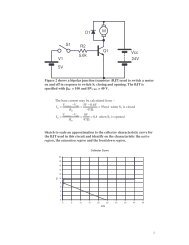
The Amplifier Stage: The amplifier is obtained using a FET. To calculate the gain of
the amplifier the transfer characteristic of the FET shown below in Fig. 9 is plotted. It
14

was assumed that the drain-source resistance of the FET is much greater than the load
so no loading takes place. A value for the transfer transconductance,
g m
, can be
obtained. This value is important since the gain of the amplifier stage above is given
by:
V
A
out
v
= −g
V
=
V
out
gs
m
V
gs
R
= −g
L
m
R
L
Fig. 9: FET circuit for obtaining transfer characteristic.
The transfer characteristic in Fig. 11 was obtained using a dc sweep with parameters
set up as in Fig. 10.
Fig. 10: DC sweep set-up.
15

Fig. 11: Transfer characteristic of FET.
Several parameters may be obtained from the transfer characteristic. The cut off
voltage is 3V and the drain to source current with gate shorted (i.e. the maximum
drain current regardless of the external circuit) is 12mA.
VG OFF
= 3V
I = 12mA
DSS
To allow a maximum drain current swing (i.e. between
I DSS
and 0) the FET is biased
at the midpoint of the curve (i.e. where
I
DSS
I
D
= ). Therefore I DSQ
is chosen to be
2
6mA. The self-bias dc load line is drawn through the Q point. The
transconductance,
g m
, is the change in drain-source current for a given change in
gate-source voltage with the drain-source voltage constant. In other words is the
inverse of the slope of the load line. Ref. [6] Appendix B
g
g
m
m
ΔI
=
ΔV
DS
GS
−3
8X10
− 4X10
=
1.26 − 0.542
−3
= 5.56mS
This FET is used in local oscillator as shown in Fig. 12 below, Fig.13 shows the
generator parameters and Fig. 14 is the response.
To calculate a value for the gain of the amplifier:
16

A
V
= g
m
R
L
= 5.56X10
−3
X1X10
3
= 5.56
The frequency of the Local Oscillator is equal to the frequency of the RF (1MHz) plus
the frequency of the IF (Already stated that the standard value is 455kHz). A
Transient Analysis was run for 10us with a print step of 1us.
Fig. 12: Local Oscillator (Amplifier Stage).
Fig. 13: LO sin wave set-up.
The peak-to-peak input voltage is 200mV and the peak-to-peak output voltage is
1.2V. This gives an amplifier gain of 6, already calculated to be 5.56. Another thing
obvious from Fig. 14 is the 180-degree phase shift.
17

Fig. 14: Input and Output Voltages of Amplifier Stage of LO.
The Feedback Network: The beta network is shown below in Fig. 15.
Fig. 15: Local Oscillator Beta Network.
Using the potential divider principle the transfer function of this network is given by:
(Note: R2 may be ignored since:
R2

1
Substituting for ω 2 = .
LC T
β =
1−
1
1
1
=
=
=
LC
1
C
2
1
+ C2
LC T
1−
C2
1−
C1C
2
C1
C
1
+ C
2
1
C
C
1
2
Let beta have a value of 0.25 then C2=4C1 (as is the case in Fig. 15 above).
Ref. [2] Appendix B
Setting up the AC sweep as shown in Fig. 16 and then zooming in on the response,
Fig. 17, the beta value can be confirmed.
Fig. 16: AC sweep.
Fig.17: AC sweep of LO feedback network.
From Fig.17 it can be seen that the resonant frequency lies at 1455kHz and that the
beta value is obtained from dividing the peak value of the input by the peak of the
output (i.e. 4), which has already been calculated by the capacitor ratio. The two
19

sections of the Local Oscillator are joined together to get our complete circuit as
shown below in Fig. 18.
Fig. 18: Local Oscillator (Amplifier stage and Beta network).
Dc conditions from the above circuit:
V
GS
= V
G
−V
S
Since there is no voltage at the input we can say that the gate voltage is 0V and that
V
the source and drain currents are equal (i.e.
I
G
S
= 0 V )
= I
D
Therefore: V
GS
= 0 −
V
S
= −I
D
R
S
From Pspice the drain current is displayed as 7.028mA.
V GS
= −7.028mX100
= −0.
7V
Since the JFET operates with the gate-source junction reverse bias the value of
I GSS
is
very small (a few nano amps) which can be obtained from data sheets. Assuming a
value of 1nA the value of the input resistance will be very large. Ref. [6] Appendix B
VGS
0.7
RIN = = = 700MΩ
−9
I 1X10
GSS
Also:
VGS
2
−3
0.7 2
I
D
= I
DSS
(1 − ) = 12X10
(1 − ) = 7. 053mA
V
3
GS OFF
20

−3
3
VD = VDD
− I
DRD
= 20V
− (7X10
X1X10
) = 13V
Since: V = I
S
D
R
S
−3
3
VDS = VD
−VS
= VDD
− I
D(
RD
+ RS
) = 20V
− 7X10
(1X
10 + 100) = 12. 3V
Fig. 19: LO output.
Fig.20: Spectrum of Local Oscillator Output.
PART 4: DESIGN OF MIXER CIRCUIT.
A mixer is a device that converts a signal from one frequency to another. Most high
frequency receivers use a mixer to down convert the received RF signal to an
intermediate frequency (IF) signal. A mixer in RF systems always refers to a circuit
21

with a non-linear component that causes sum and difference frequencies of the input
signals to be generated. The mixer is achieved by applying the Local Oscillator (LO)
signal to one mixer port and the Radio Frequency (RF) signal to the other port. As can
be seen in Fig. 21 below the inputs are linearly added by a FET (when suitably biased
produces second order non linear device). The current and voltage are related by the
quadratic relationship:
in
2
in
i = av + bv + cv
Where the input voltage can be expressed:
3
in
.......
v
in
= v
LO
cos ω t + v
LO
RF
cosω
RF
t
If we substitute this into the previous equation the squared term will produce the
cosAcosB term which when expanded,
cos ω t & cosω
t generate sum and
LO
RF
difference frequencies. All other frequencies are filtered out using a parallel tuned LC
circuit resonant at the desired intermediate frequency:
f
IF
=
f
LO
−
f
RF
Ref. [1]& Ref. [7] Appendix B
This tuned circuit will be added in the final design but for the purpose of testing Fig.
21 will just have a 1k resistor as its load.
The mixer uses a JFET as configured in the local oscillator. Using dc formulae
previously stated and using Pspice to get values for the gate and source voltages and
drain current (using a 20V-power source).
VGS = VG
−VS
= 4 .872uV
− 2.116V
= 2. 12V
Similarly: VGS = −I
D
RD
= −1 .058mX
2k
= 2. 12V
Other voltages:
And checking:
V
V
V
D
S
DS
= V
= I
DD
D
= V
R
DD
− I
S
D
= 1.058mX
2k
= 2.116V
− I
D
R
D
( R
= 20 −1.058mX1k
= 18.94V
D
+ R
S
) = 17.88V
VGS
2 2.12 2
I
D
= I
DSS
(1 − ) = 12m(1
− ) = 1. 033mA
V
3
GS OFF
22

Ref. [6] Appendix B
Fig. 21: Mixer circuit.
In the mixer circuit above Vrf stands for the RF voltage (connected to the gate) and
Vlo stands for the LO voltage (connected to the source). Therefore, Vrf has a
frequency of 1MHz and the Vlo has a frequency of 1455kHz. The transient analysis
on the mixer circuit gives the response shown below in Fig. 22.
Fig. 22: Mixer Output.
The spectrum of the mixer is shown in Fig. 23.
23

Fig. 23: Mixer Spectrum.
It can be observed from the spectrum in Fig. 35 that the desired signal is located at
455kHz. All the other spectral components will be filtered out as previously stated
with the tuned LC circuit. The desired signal will be fed to the IF stages, both of
which will be tuned to 455kHz and will have a bandwidth as close to 10kHz as
possible to ensure no desired information will be lost.
PART 5: DESIGN OF IF STAGE.
The output of the Mixer is amplified by two IF amplifier stages. Most of the receiver
sensitivity and selectivity is to be found in the IF stage. The two IF stages are tuned to
f IF
(= 455kHz). The highly amplified IF signal will then be applied to the Detector
where the original modulating signal is recovered. The IF amplifier is configured
using a BJT with a double tuned load. Consider the tuned LC circuit.
If Q>10 then we can approximate:
1
f
O
≈
2π
LC
1
∴C
≈
2
4π
f
2
O
= 455kHz
F
L
Choosing L=175uH then we get C=700pF from above. (Note: we also add in a small
resistance of 10 Ohms in series with the inductor).
Ref. [1] Appendix B
24

Values for the second LC tuned circuit have to be calculated. The reason the double
tuned circuit is used is to get a flat top response for the amplifier at the resonant
frequency. The single-tuned response has a very sharp response, which could lead to
the loss of information. However, using double-tuned circuits means a coupling coefficient,
k c
, has to be used. The inductance and capacitance values used in the single
tuned circuit are referred to as L2 and C2 respectively. Values for L1 and C1 are
calculated. As before the L value is chosen (L1=210uH) and the corresponding C
value to resonate at 455kHz is C2=582pF.
Ref. [3] Appendix B
Changing the resonant frequency to radian seconds gives
ω
O
6 −1
= 2.863X10
rs
Calculating the Q factor for the two circuits:
Q
Q
U1
U 2
6
ω
O
L1
2.863X10
X 210X10
= =
r1
20
6
ω
O
L2
2.863X10
X175X10
= =
r2
10
Calculating the primary and secondary windings:
−6
−6
= 30
= 50
Q
S
= Q U 2
= 50
The primary winding has to take into account Qc:
Q
= R
C
ω
O
C1
= 80X10
3
X 2.863X10
6
X 582X10
−12
= 133.3
Q
P
⎡ 1
= ⎢
⎣QU
1
1
+
Q
C
⎤
⎥
⎦
−1
⎡
= ⎢
⎣
1
30
+
1
133.3
⎤
⎥
⎦
−1
= 24.49
A value for the critical coupling co-efficient is obtained:
k
k
C
C
=
Q
1
P
Q
S
= 0.02858
=
1
24.49X
50
The circuit diagram for the IF stage is shown below in Fig. 24.
25

The BJT used in the IF amplifier is the same as that used in RF amplifier and will use
the same formulae for its dc conditions.
β
DC
(i.e. dc current gain of the transistor) using current values from Pspice:
β
DC
=
I
I
C
B
3.23mA
= = 20.1
160.42uA
This is a much smaller value than the corresponding value in the RF amplifier, but it
is still an acceptable value.
α
DC
=
I
I
C
E
3.23mA
= = 0.995
3.247mA
This is the same as the RF amplifier.
V
V
I
B
E
E
R2
50k
= VDD
= 20V
R1
+ R2
80k
+ 50k
= V −V
= (7.7 − 0.7) V = 7V
B
V
=
R
E
E
BE
7V
= = 3.5mA
2kΩ
= 7.7V
Pspice gives values for the base and emitter voltages as 7.167V and 6.494V
respectively and emitter current as 3.247mA.
The internal resistance of the transistor:
25mV
r ' e = = 7. 14Ω
I E
The load resistance:
−6
L 210X10
R = =
= kΩ
L −
CR 582X10
X 20
18
12
S
L1
VO
RL
Voltage gain: A = = =
C1Rs
V
= 2521
V r'
e r'
e
IN
The voltage gain expressed in dBs: 20log(2521) = 68dB.
Power gain = current gain X voltage gain = 20.1 X 2521 = 50672.
Input Impedance of the transistor:
VB
7.167V
RIN = = = 420kΩ
I 17.08uA
B
R
Total
IN IN
7
= R1
R2
R = 80k
50k
420k
= 28. kΩ
Ref. [6] Appendix B
26

Fig. 24: Double tuned IF amplifier.
The AC sweep run on Fig.24 gives the response in Fig. 25.
Fig. 25: Zooming in on response to measure BW of IF stage.
The response shows that the –3dB bandwidth is 12kHz. The desired BW is 10kHz to
pass the desired signal. The gain lies at just above 46dB. This IF amplifier will be
used twice in the hierarchy structure (i.e. the two IF stages in the final design will
have the same component values). This highly amplified and highly selected signal
will now be fed to the AM detector circuit with AGC (Automatic Gain Control).
PART 6: AM DETECTION WITH AGC.
27

For the purpose of testing the detector circuit the AM wave generator previously
developed is applied to the envelope detector. However, the value of the feedback
resistor will be increased from 150 Ohms to 500 Ohms. The reason for this is to
increase the minimum carrier amplitude to above 200mV since the minimum cut-in
voltage for a germanium diode is 200mV. If the minimum amplitude were below
200mV then the diode would not be turned on. With this in mind the diode
rectification circuit is shown below in Fig.26.
Fig. 26: Diode rectification.
Fig. 27 displays the originally generated AM wave and the rectified version of the
wave.
Fig. 27: Rectified AM signal.
Zooming in on a small portion of the waveforms displays the effect of rectification
more clearly, see Fig. 28.
28

Fig. 28: Enlarged section of diode rectification.
It can be seen from Fig. 28 that the negative part of the rectified version is
suppressed. The next step is to filter out undesired RF components such as the carrier,
by adding in a capacitor in parallel with the resistor. The reason for this is during the
positive cycle of the AM wave the diode is forward biased and the capacitor charges
up to the peak value. A ripple will occur as the capacitor discharges through the
resistor during the time period between the peaks of the AM wave. One solution
would be to increase the RC time constant. It must also take into consideration that if
the RC time constant is too large the voltage across the capacitor will be unable to
follow the rate at which the envelope is decreasing and result in the loss of
information. The following formula is used to ensure this doesn’t happen, the
optimum value for the capacitor is given by:
C ≤
1
m 2
−1
2 R L
≤
π f
MAX
m MAX
11.73nF
Where the maximum modulating frequency is 5kHz, the modulating index is 0.5 and
choosing a resistor value of 4.7k Ohms. A low pass RC filter is added to ensure there
is no RF ripple entering the audio amplifier. There is a second low pass RC filter for
the purpose of AGC (see Fig. 29).
29

Fig. 29: AM detector circuit with AGC.
The main function of the AM detector is to recover the modulated signal. It has
another function called automatic gain control (AGC). AGC is required in the
superhetrodyne receiver to regulate the receiver gain as the input carrier amplitude
varies due to a variety of reasons. Since these variations are very slow the low pass
filter for the AGC has a very low cut off frequency (i.e. 1Hz). Choosing a resistor
value of 100kOhms we get:
1
f
AGC
= = 1Hz
2πRC
1
C = = 1.59uF
2πf
R
AGC
Ref. [2] Appendix B
Choosing a resistor value of 400kOhms for the audio out low pass filter with a
resonant frequency of 10kHz:
1
C =
2 π f
audio
R
= 39.79 pF
However this capacitor is very small and is the order of stray capacitance. Choosing
R=100kOhms gives C= 0.159nF. This will be implemented in the hierarchy structure.
Note: the reason the resistor values are chosen at 100k is they are much larger than the
resistor value in the CR high pass filter at the amp output to avoid loading the circuit.
Fig. 30 below shows the AGC and audio signals.
30

Fig. 30: AGC and audio signals.
The AGC signal should be constant. From Fig. 30 it can be seen to sit at dc and it
varies by a slight amount (in the order of milli-volts).
PART 7: DESIGN OF PRE-AMPLIFIER AND POWER AMPLIFIER.
Class A, B, and C amplifiers are used in transmitters. Class A amplifiers are used in
low-power stages where device dissipation and efficiency are not critical. Class B and
C amplifiers are used where high power and efficiency are required. In the
superhetrodyne receiver the pre-amplifier stage and power amplifier stage are
combined and implemented together as an audio amplifier. Therefore, class C
amplifiers cannot be used in audio amplifiers because the output current flows for less
than one-half of the input signal cycle. Class B operation is achieved when the active
device (in this case the BJT) is biased at cut-off, so that the output current will flow
for only one half of the input signal cycle. Efficiency can reach as high as 78.5% and
for linear system operation must be used in a push-pull circuit configuration. Fig. 31
below shows the circuit of the audio amplifier using a class B output stage.
Ref. [4], Ref. [5] & Ref. [6] Appendix B
31

Fig. 31: Audio amplifier.
Dc conditions (with 20V-power supply):
I
C 3.623mA
BJT Q9 (pre-amplifier stage): β
DC
= = = 167. 5
I 21.63uA
B
α
DC
= 0.994
I E
= 3.64mA
r'
e = 6.9Ω
I
C 3.817mA
BJT Q10 (below diodes): β
DC
= = = 14. 7
I 260.1uA
B
α
DC
= 0.994
2k
V B
= 20 = 3. 33V
(Pspice value = 2.9V)
(10 + 2) k
V E
= 3 .33 − 0.7 = 2. 63V (Pspice value = 2.128V)
I E
= 2.63mA
r'
e = 9.5Ω
I
C 21.89mA
BJT Q11 (npn transistor in power amp): β
DC
= = = 162
I 135.1uA
B
α
DC
= 0.994
32

I
C 22.02mA
BJT Q12 (pnp transistor in power amp): β
DC
= = = 5. 8 (very low value)
I 3.817mA
α = 1.21 (Note: this should be less than 1)
DC
B
Ref. [6] Appendix B
Fig. 32: Audio amplifier input and output voltage waveforms.
Fig. 32 displays the input and output voltage waveforms. From this the voltage gain
of the amplifier can be measured as 13, since a 100mV input signal produces a 1.3V
output waveform. Since this is a power amplifier the power is an important parameter.
Fig.33 plots the load power and the average load power.
Fig. 33: Audio amplifier load power and average load power.
33

Fig. 33 gives the average load power as just below 2.2mW and having a peak value of
just under 4.5mW.
Fig. 34: Load current of audio amplifier.
Fig.34 shows the load current of the amplifier, having a max value of 6.5mA.
CHAPTER 4: FINAL TESTS AND RESULTS (HIERARCHY
STRUCTURE).
With the superhetrodyne receiver designed, tested and simulated in its various blocks
a top-down approach with hierarchical methods in Pspice is used to simulate the
complete circuit. Fig. 35 below shows the main block of the superhetrodyne receiver.
Fig. 35: Hierarchy main block.
34

The middle section of the hierarchy design consists of eight blocks as shown in Fig.
36, each block contains one sub-circuit of the receiver.
Fig. 36: Hierarchy middle block.
Each of the previously designed and simulated circuits are built inside the middle
block. Figs. 37-44 show these circuits.
Fig. 37: Block 1 – AM generator.
35

Fig. 38: Block 2 – RF amplifier.
Fig. 39: Block 3 – Mixer.
36

Fig. 40: Block 4 – Local oscillator.
Fig. 41: Block 5 – IF1.
37

Fig. 42: Block 6: IF 2.
Fig. 43: Block 7 – AM detector & AGC
38

Fig. 44: Block 8 – Audio amplifier.
A couple of component changes had to made in the hierarchy structure:
Block 1- AM generator: The feedback resistor is increased up to 1k so as it is the
same as the input resistors and the CR high-pass filter at the output changed to a
100nF capacitor and a 20k resistor. The image frequency is also added in. This has a
frequency of 1910kHz, as previously defined, and an amplitude the same as the
carrier.
Block 3 – Mixer: As previously stated an LC circuit tuned to 455kHz replaces the
load resistor.
1
1
f
s
= =
455kHz
2 LC
=
Re −6
−9
π 2π
10.49X10
X11.66X10
Block 4 - LO: the inductor in the feedback network is reduced slightly to 33.5uH to
fix resonance at 1.455kHz.
Block 6 - IF2: input resistors reduced to 8k and 5k and a small base resistance of 10
Ohms is added in.
39

Block 7 – AM detector: as previously stated the resistor in the audio CR filter is set at
100k as to increase the capacitor value to avoid stray capacitance. The capacitor at the
input is reduced to 1nF, which is acceptable as the max value is11.73nF.
Loading effects: the main problem associated with the hierarchy structure is the
loading effects between the hierarchy blocks. It is essential to isolate the blocks from
each other to avoid one block loading down the entire circuit and effectively stopping
the receiver from working. The solution in Pspice is through transformers. Setting the
inductor values in the transformer to L1=20uH and L2=0.3uH and a coupling of
0.9999 (i.e. practically 1) a step down transformer is achieved.
As can be seen from Figs. 37-44 above transformers are placed in the following
places:
(1) A step down transformer is placed at the input of the RF amplifier (see
Fig. 38) to avoid the 20k resistor from the AM generator being in parallel
with the input resistance of the RF amplifier.
(2) Another transformer is placed at the RF output (see Fig. 38) to avoid
loading with the mixer. For convenience and design reasons this
transformer is placed here and not at the input of the mixer because it
incorporates the inductor from the tuned LC circuit in the RF load.
(3) A transformer is used to couple the LO signal into the mixer (see Fig. 39).
(4) The input of the first IF stage has a transformer (see Fig. 41) to avoid
loading between the tuned LC circuit in the mixer load and input resistance
of the IF amplifier.
(5) The IF amplifier is a double tuned circuit and hence has two inductors in
the load. Therefore these can be implemented as a transformer also to
avoid loading effects between the two IF stages (see Fig. 41).
40

The first major test for the superhetrodyne receiver is how well the RF amplifier
rejects the image frequency. Fig 45 below plots the AM and RF spectra with the
image frequency and zooms in to view the image frequency at the RF output. It
can be seen that the image frequency greatly distorts the AM spectrum. However,
viewing the RF spectrum it is seen that the carrier frequency (1MHz) is amplified
from 46.2mV to 400mV, whereas the image frequency is reduced from 24.8mV to
8.6mV. Other frequencies are almost completed attenuated. The image frequency
2
rejection ratio is calculated: 20 log[1 + Q 2 γ ]
f
image f
RF 1.91M
1M
Where γ = − = − = 1. 39
f f 1M
1.91M
RF
image
2 2
Therefore the image frequency rejection ratio is: 20 log[1 + 100 X1.39
] = 85. 68
Fig. 45: AM and RF spectra.
Fig. 46 below shows the development of the AM wave throughout the
superhetrodyne receiver.
41

Fig. 46: AM signal in superhetrodyne receiver.
Taking a look at the Fourier transform in Fig. 47 displays the two signals going
into the mixer and the sum and difference frequencies in the mixer output.
Fig. 47: Mixer spectrum.
Although the mixer load is tuned to 455kHz the spectrum above shows spectral
peaks decreasing in amplitude at 910kHz, 1MHz, 1.455MHz, 1.91MHz, 2MHz,
2.455MHz etc. There is also an unwanted spectral peak at 555kHz. The only
possible reason for this is that the image frequency is causing distortion in the
42

spectrum. However, as long as the IF stages are correctly tuned and have
sufficient gain the difference frequency will be selected and amplified while the
other frequencies attenuated. This is viewed in the IF spectra below in Fig. 48.
Fig. 48: IF spectra.
The difference frequency (i.e. the desired frequency) has an amplitude of 40mV at
the output of the mixer. This is now applied to the two IF amplifiers. The output
of the first IF stage shown in the second plot of Fig. 48, it is noted that the
difference frequency lies at 600mV at this stage. This implies that IF1 has a gain
of 15. The third plot of Fig. 48 displays the output of the second IF stage. At this
point the difference frequency is now at 12.6V. The second IF stage has a larger
gain than the first stage (i.e. 12.6V/600mV = 21). A very important feature that
can be seen from Fig. 48 is that all other frequencies apart from the selected one
are greatly attenuated by the IF amplifiers.
The AM detector has the function of detecting this highly amplified IF signal. As
can be seen from the sixth plot of Fig. 46 previously the AM detector begins to
trace or “detect” the IF signal. The detector has diode rectification at its input and
the first plot on Fig. 49 below shows the rectification of the signal at 455kHz with
43

an amplitude of 538mV. The output is fed through a high pass filter as shown in
the second plot. This signal with a 6.83mV amplitude is fed to the audio amplifier
where it is amplified up to 79.35mV. The AM signal generated at the start had an
amplitude of 72mV and now at the output it has a value of 79.35mV.
Fig. 49: AM detection and audio spectrum.
Zooming in on the low frequency components of the AM detector spectrum, as in
Fig. 50 below, a spectral component is present at 5kHz, which has amplitude of
14mV. The reason this component is very important is that 5kHz is the
modulating frequency. This frequency is required to be amplified by the audio
amplifier. This is the case in Fig. 51, where the modulating frequency is amplified
up to 470mV.
44

Fig. 50: Modulating frequency in AM detector spectrum.
Fig. 51: Modulating frequency in audio spectrum.
It must be noted that the modulating frequency lies at a much higher amplitude
than the difference frequency at the output of the audio amplifier. The modulating
frequency (i.e. at 5kHz) has an amplitude of 470mV and the difference frequency
(i.e. at 455kHz) only has an amplitude of 79mV.
45

CHAPTER 5: CONCLUSIONS.
* One of the things that I have learned personally from this project is to adopt a
methodical approach to problem solving. From the outset of the project the
aim was to design and simulate a complete superhetrodyne receiver. Rather
than tackle the problem in one large section, the superhetrodyne receiver was
looked at in block diagram form. Each block was designed and tested
separately to ensure each individual circuit worked correctly prior to
simulating the complete circuit. This practical approach to problem solving
enabled diagnosis of errors and faults to exact locations and solving of
problems was therefore easier.
* The aim of this project was to design and simulate a complete superhetrodyne
receiver using Pspice. Knowledge of analogue design of circuits greatly
helped in the design of the project. DC formulae and circuit configurations
studied in the process of three years of Electronics gave good background
knowledge of the type of circuits to be implemented in the superhetrodyne
receiver. Another aspect that helped was the previous use of the Pspice
simulation package. Now having spent the duration of the project working
with Pspice I would have to say that my knowledge of the package has been
greatly enhanced, as too is my understanding of amplifiers and other circuits
in general.
* One thing that was helpful in some of the solving of problems and errors,
especially with the RF and IF stages, was viewing the dc conditions of the
circuit with the aid of Pspice. Often component values had to be changed and
viewing voltages and currents in circuits ensured that the component values
were reasonable. Many simulation errors occurred due to unrealistic dc
conditions in circuits.
46

* Working on the IF stages of the design provided a problem is so far as that the
main objective of this stage to provide good selectivity. Selectivity is best
achieved at low frequencies, especially when using tuned LC circuits.
However, the problem arises when low frequencies lead to interference and
distortion due to what is known as image frequencies. This is when two
signals are received that differ by twice the intermediate frequency.
If we have an image frequency:
f = f + 2 f
image
RF
IF
Where
f RF
is the desired frequency.
Mixing the image frequency with
f
LO
, where
f = f + f , will give:
LO
RF
IF
f = f ±
IF
image
f
LO
Taking the difference frequency:
f
IF
=
f
image
−
f
LO
Therefore the difference frequency is:
= ( f + 2 f ) − ( f + f )
=
f
IF
RF
IF
RF
IF
Therefore the image frequency generates a signal at
f IF
also.
* The selection of the Q values in the RF and IF blocks was very important as an
engineering compromise occurs. High selectivity is required which can be
achieved with LC circuits with high Q values. However, circuits with high Q
values have narrower bandwidths. It must be taken into consideration that the
bandwidth must be large enough to pass all the information (i.e. the carrier and
both sidebands).
* Undoubtedly, the biggest conclusion to be drawn from the project is in the
area of loading. In the hierarchy design the major problems in simulation of
the circuit were due to the loading effects from one hierarchy block to another.
Inspection of the overall design showed that some parts of the design were
suppressing other parts and preventing them from functioning correctly. The
47

solution was the use of transformers between circuits to avoid one circuit
loading down another.
* An observation with the Pspice program is that it tends to cling to or hold on
to values after component values are changed. Looking at voltages and
currents through the circuit sometimes showed impossible results and the only
conclusion was that Pspice was still reading previous values for voltages,
currents and component parts even after alterations had been made in the
circuit.
* The main aim of the project was to design and simulate the complete
superhetrodyne receiver. The results of the project can be summarised as
follows: an AM wave was generated with a carrier frequency of 1MHz and a
modulating frequency of 5kHz (i.e. a 10kHz bandwidth). The carrier had an
amplitude of 732mV. The AM signal was fed to an RF amplifier. The image
frequency, set to 1.91MHz, was greatly attenuated at the RF stage. A signal
was generated at the local oscillator stage and when “mixed” or heterodyned
with the RF signal produced the difference or intermediate frequency, which
had an amplitude of 40mV. This difference frequency at 455kHz was
amplified by two IF stages (most of the sensitivity and selectivity found here).
The signal was amplified to a value of 12.6V. The AM detector now detected
this signal. The detector also detected the modulating frequency at 5kHz. The
audio amplifier amplified the difference frequency up to 79.35mV and the
modulating frequency up to 470mV.
In conclusion, although the overall final design did not work completely I feel
good progress was made throughout the project. All of the separate blocks
worked individually but when implemented into a hierarchical structure
problems arose. The biggest problem as previously stated was with loading
effects. The use of transformers and coupling capacitors (in which the values
48

are very important) combated this problem. Even with this solved Pspice still
didn’t simulate the complete circuit as expected. These maybe due to the
Pspice package itself, with regards to the installation of the program.
However, it must be concluded that some aspects of the final design were
satisfactory even though a sine waveform was not recovered at the detector.
The image frequency was attenuated sufficiently by the RF amplifier. The LO
produced a signal which mixed with the RF signal. The IF stages provided
good selectivity and gain. Also, the detector detected the IF signal and a signal
at the modulating frequency which were then amplified by the audio amplifier.
So although not a complete success I feel this project was very beneficial and
satisfactory.
APPENDIX A: SOFTWARE USED.
Pspice Release, Version 8
By MicroSim.
Paint Shop Pro, Version 4
By JASC, Inc.
Microsoft Word 2000
By Microsoft Corporation.
Microsoft Equation Editor, Version 3.0
By Microsoft Corporation.
APPENDIX B: REFERENCES.
Ref. [1] “Communication Engineering Theory Notes”
By Paul Tobin for third year degree in Applied Electronics (SEE3).
Ref. [2] “Pspice Lab Manual”
By Paul Tobin for third year degree in Applied Electronics (SEE3).
49

Ref. [3] “Electronic Communication Techniques, Forth Edition”
By Paul Young (Publ. Prentice Hall).
Ref. [4] “Pspice for Windows, A Circuit Simulation Primer”
By Roy W. Goody (Publ. Prentice Hall).
Ref. [5] “Pspice for Windows, Volume 2, Operational Amplifiers & Digital
Circuits”
By Roy W. Goody (Publ. Prentice Hall).
Ref. [6] “Electronic Devices, Fifth Edition”
By Thomas L. Floyd (Publ. Prentice Hall).
Ref. [7] “Radio Communication”
By D. C. Green (Publ. Longman).
Ref. [8] http://my.integritynet.com.au/purdic/am_rec.htm
By Ian Purdie.
Ref. [9] http://www.ezlink.com/~crash/parks/hetbasic.html#modulate
Link: www.googgle.com
APPENDIX C: SCALE SUFFIXES
Symbol Scale Name
f 10e-15 Femtop
10e-12
Picon
10e-9 Nanou
10e-6 Microm
10e-3 Millik
10e+3 Kilo-
M 10e+6 Mega-
G 10e+9 Giga-
T 10e+12 Tera-
APPENDIX D: SCHEMATICS & PROBES.
Schematics:
Fig. 3: Amplitude Modulator.
Fig. 6: Single tuned RF amplifier.
Fig. 9: FET circuit for obtaining transfer characteristic.
Fig. 12: Local Oscillator (Amplifier Stage).
Fig. 15: Local Oscillator Beta Network.
50

Fig. 18: Local Oscillator (Amplifier stage and Beta network).
Fig. 21: Mixer circuit.
Fig. 24: Double tuned IF amplifier.
Fig. 26: Diode rectification.
Fig. 29: AM detector circuit with AGC.
Fig. 31: Audio amplifier.
Fig. 35: Hierarchy main block.
Fig. 36: Hierarchy middle block.
Fig. 37: Block 1 – AM generator.
Fig. 38: Block 2 – RF amplifier.
Fig. 39: Block 3 – Mixer.
Fig. 40: Block 4 – Local oscillator.
Fig. 41: Block 5 – IF1.
Fig. 42: Block 6: IF 2.
Fig. 43: Block 7 – AM detector & AGC
Fig. 44: Block 8 – Audio amplifier.
Probes:
Fig. 4: The AM signal.
Fig. 5: Enlarged section of the AM spectrum.
Fig. 7: RF amplifier response.
Fig. 8: Zoom in to measure bandwidth.
Fig. 11: Transfer characteristic of FET.
Fig. 14: Input and Output Voltages of Amplifier Stage of LO.
Fig.17: AC sweep of LO feedback network.
Fig. 19: LO output.
Fig.20: Spectrum of Local Oscillator Output.
Fig. 22: Mixer Output.
Fig. 23: Mixer Spectrum.
Fig. 25: Zooming in on response to measure BW of IF stage.
Fig. 27: Rectified AM signal.
Fig. 28: Enlarged section of diode rectification.
Fig. 30: AGC and audio signals.
Fig. 32: Audio amplifier input and output voltage waveforms.
Fig. 33: Audio amplifier load power and average load power.
Fig. 34: Load current of audio amplifier.
Fig. 45: AM and RF spectra.
Fig. 46: AM signal in superhetrodyne receiver.
Fig. 47: Mixer spectrum.
Fig. 48: IF spectra.
Fig. 49: AM detection and audio spectrum.
Fig. 50: Modulating frequency in AM detector spectrum.
Fig. 51: Modulating frequency in audio spectrum.
Others:
Fig. 1:The block diagram of the Superheterodyne receiver.
Fig. 2: Generator Parameters.
Fig. 10: DC sweep set-up.
Fig. 13: LO sin wave set-up.
Fig. 16: AC sweep.
51