ieee transactions on very large scale integration (vlsi) - Computer ...

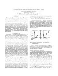
YANG et al.: EXTRACTION ERROR MODELING AND AUTOMATED MODEL DEBUGGING IN HIGH-PERFORMANCE CUSTOM DESIGNS 771
the is updated by copying to the
column which is main-indexed with (line 12). Intuitively, the
columns of
under the same main index contain
the values of the PIs prior to the last indexed clock triggered. Finally,
the is updated with the input vector (line 16).
In our implementation, we use a parallel bitwise implementation
for both the storage tables and for the simulation retrieving as
many test vectors as the length of the computer word [9].
The values stored in the tables are used appropriately by
ENHANCED_PATH_TRACE to restore logic values in the core circuitry
and assist path-trace during diagnosis. When path-trace
marks the registers in register layer II, it reads the proper entry
in
and retrieves the correct values in combinational
circuitry B by simulating the circuitry with the values
read from the table. Then, path-trace proceeds by marking in
the combinational circuitry B (lines 24–26). When it reaches
the registers in register layer I, it again reads the entry in
according to clocks controlling the registers on
the path and restores the states of the lines in combinational
circuitry A. Path-trace continues marking in core circuitry A
and terminates when it reaches a primary input of the circuit,
as explained earlier. These actions are taken in lines 29–31.
The above procedures are utilized when no state equivalence
information is available. In the cases of partial and full state
equivalence, path-trace can start marking from erroneous primary
outputs as well as memory elements that propagate erroneous
logic values and their state equivalence information is
available. We omit this code which is a straightforward extension
of the one presented earlier.
In the final paragraphs of this section, we analyze memory
requirements for the various tables. In this analysis, we partition
the circuit to allow the primary input to be at stage 0, the register
layer I at stage 1, and so on. We also assume that, for stage
, there are memory elements (primary inputs) and local
clocks.
Using the above notation, it can be shown that the size
(i.e., number of table entries) of the largest table at stage
is , where is the maximum number of
pipeline stages. Recall that each stage maintains additional
smaller tables for all subsequent stages. Therefore, the
size of the total number of tables at stage is found to be
. Using this result, the total number of
tables for the complete design is .
To further analyze the memory requirements as the number of
pipeline stages increases, for the sake of simplicity, we assume
that the number of registers and the number of local clocks for
each register layer in every pipeline stage is upper bounded by
and , respectively. In other words, and ,
. Using this upper bound, the total number of table entries
is
. It can be seen that, for every increase
in the number of pipeline stages , the number of table entries
increases roughly by factor of . For example,
, and so on,
or, in general, .
It is seen that the size of the table entries relates to the number
of clocks per pipeline stage and the total number of pipeline
stages in an exponential manner, a fact that may require prohibitive
amounts of memory for large industrial designs with
very deep pipelines. This is expected since the algorithm handles
a sequential model with no state equivalence information
to the transistor level. However, in practice, deep pipelines are
usually designed in blocks of smaller (pipelined) stages to ease
test generation, verification etc [15]. Additionally, the number of
local clocks and the number of pipeline stages is a small fraction
to the total number of circuit lines. Finally, the trend today
in high-performance designs is multithreading on small-sized
pipelines due to power and reliability concerns. Therefore, in
most practical cases, the debugging algorithm is expected to be
memory efficient.
B. -Simulation
In most model-dependent diagnosis algorithms, the effects
of the faults/errors are explicitly specified [9], [14]. During
diagnosis, a model-dependent algorithm usually performs one
logic simulation step for every error model manifestation on
each suspect line. Therefore, this type of diagnosis is more
suitable for simple faults/errors where their effects are easy to
enumerate [14]. For example, the effects of a stuck-at fault are
modeled with only two values 0 and 1 and, for each suspect line
, the algorithm can perform two simulations, stuck-at-0 and
stuck-at-1. to see the effects of the candidate fault. However,
for complicated faults/errors, such as the extraction errors
presented here, the cardinality of the error models may be large,
and it may be computationally expensive to simulate each
such effect during diagnosis. In this case, model-free diagnosis
seems to serve better in tackling the problem [14].
Model-free diagnosis simulates a logic unknown value
on candidate error lines to capture all possible paths for error
propagation [14]. In the proposed debugging algorithm, after
path-trace returns a set of candidate error locations, the algorithm
performs this -simulation step using failing input test
vectors. Because of multiple error sites in the netlist, the true
candidate error locations must be marked by path-trace at least
times, where is the cardinality of failing input test
vectors and is the number of erroneous module instantiations.
This claim is proved in terms of a simple theorem in [14] using
the pigeon-hole principle, and we refer the reader to that paper
for details. Furthermore, recall that these multiple error sites are
instances of one single module. In other words, we can prune the
size of the candidate list further using the following rule. The
sum of path-trace marks for all instantiations of a candidate
error module must be greater or equal to . -simulation is
performed on modules that qualify this rule.
Since some error types involve the logic unknown , we introduce
a second unknown value and simulate this value on
the candidate error locations. Under this scenario, if a gate primitive
has an input with controlling value, then this input prevails,
otherwise value prevails over any other input. For example,
a two-input gate with fan-in values of 0 and evaluates
to 0 while one with values and or 1 and evaluates to
. A module qualifies for correction if this simulation of the
value propagates to all erroneous primary outputs [14].