The calculation of CCT diagrams for engineering steels.pdf - LFS
The calculation of CCT diagrams for engineering steels.pdf - LFS
The calculation of CCT diagrams for engineering steels.pdf - LFS

You also want an ePaper? Increase the reach of your titles
YUMPU automatically turns print PDFs into web optimized ePapers that Google loves.
Archives<br />
<strong>of</strong> Materials Science<br />
and Engineering<br />
Volume 39<br />
Issue 1<br />
September 2009<br />
Pages 13-20<br />
International Scientific Journal<br />
published monthly by the<br />
World Academy <strong>of</strong> Materials<br />
and Manufacturing Engineering<br />
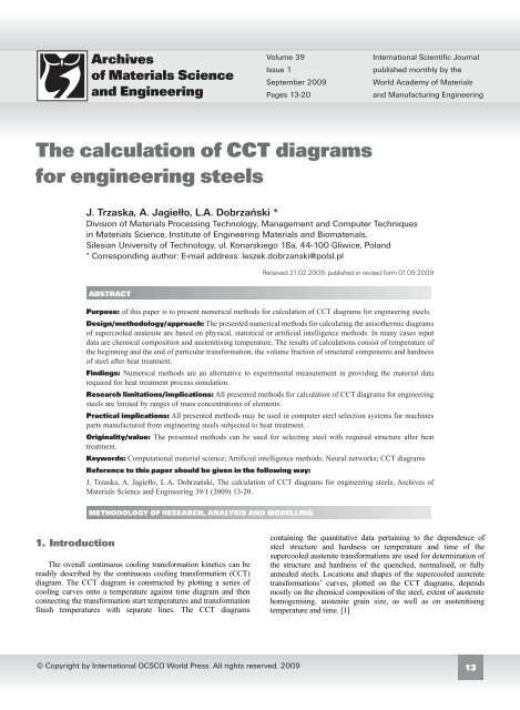
<strong>The</strong> <strong>calculation</strong> <strong>of</strong> <strong>CCT</strong> <strong>diagrams</strong><br />
<strong>for</strong> <strong>engineering</strong> <strong>steels</strong><br />
J. Trzaska, A. Jagie³³o, L.A. Dobrzañski *<br />
Division <strong>of</strong> Materials Processing Technology, Management and Computer Techniques<br />
in Materials Science, Institute <strong>of</strong> Engineering Materials and Biomaterials,<br />
Silesian University <strong>of</strong> Technology, ul. Konarskiego 18a, 44-100 Gliwice, Poland<br />
* Corresponding author: E-mail address: leszek.dobrzanski@polsl.pl<br />
Received 21.02.2009; published in revised <strong>for</strong>m 01.09.2009<br />
ABSTRACT<br />
Purpose: <strong>of</strong> this paper is to present numerical methods <strong>for</strong> <strong>calculation</strong> <strong>of</strong> <strong>CCT</strong> <strong>diagrams</strong> <strong>for</strong> <strong>engineering</strong> <strong>steels</strong>.<br />
Design/methodology/approach: <strong>The</strong> presented numerical methods <strong>for</strong> calculating the anisothermic <strong>diagrams</strong><br />
<strong>of</strong> supercooled austenite are based on physical, statistical or artificial intelligence methods. In many cases input<br />
data are chemical composition and austenitising temperature. <strong>The</strong> results <strong>of</strong> <strong>calculation</strong>s consist <strong>of</strong> temperature <strong>of</strong><br />
the beginning and the end <strong>of</strong> particular trans<strong>for</strong>mation, the volume fraction <strong>of</strong> structural components and hardness<br />
<strong>of</strong> steel after heat treatment.<br />
Findings: Numerical methods are an alternative to experimental measurement in providing the material data<br />
required <strong>for</strong> heat treatment process simulation.<br />
Research limitations/implications: All presented methods <strong>for</strong> <strong>calculation</strong> <strong>of</strong> <strong>CCT</strong> <strong>diagrams</strong> <strong>for</strong> <strong>engineering</strong><br />
<strong>steels</strong> are limited by ranges <strong>of</strong> mass concentrations <strong>of</strong> elements.<br />
Practical implications: All presented methods may be used in computer steel selection systems <strong>for</strong> machines<br />
parts manufactured from <strong>engineering</strong> <strong>steels</strong> subjected to heat treatment.<br />
Originality/value: <strong>The</strong> presented methods can be used <strong>for</strong> selecting steel with required structure after heat<br />
treatment.<br />
Keywords: Computational material science; Artificial intelligence methods; Neural networks; <strong>CCT</strong> <strong>diagrams</strong><br />
Reference to this paper should be given in the following way:<br />
J. Trzaska, A. Jagiełło, L.A. Dobrzański, <strong>The</strong> <strong>calculation</strong> <strong>of</strong> <strong>CCT</strong> <strong>diagrams</strong> <strong>for</strong> <strong>engineering</strong> <strong>steels</strong>, Archives <strong>of</strong><br />
Materials Science and Engineering 39/1 (2009) 13-20.<br />
METHODOLOGY OF RESEARCH, ANALYSIS AND MODELLING<br />
1. Introduction<br />
<strong>The</strong> overall continuous cooling trans<strong>for</strong>mation kinetics can be<br />
readily described by the continuous cooling trans<strong>for</strong>mation (<strong>CCT</strong>)<br />
diagram. <strong>The</strong> <strong>CCT</strong> diagram is constructed by plotting a series <strong>of</strong><br />
cooling curves onto a temperature against time diagram and then<br />
connecting the trans<strong>for</strong>mation start temperatures and trans<strong>for</strong>mation<br />
finish temperatures with separate lines. <strong>The</strong> <strong>CCT</strong> <strong>diagrams</strong><br />
containing the quantitative data pertaining to the dependence <strong>of</strong><br />
steel structure and hardness on temperature and time <strong>of</strong> the<br />
supercooled austenite trans<strong>for</strong>mations are used <strong>for</strong> determination <strong>of</strong><br />
the structure and hardness <strong>of</strong> the quenched, normalised, or fully<br />
annealed <strong>steels</strong>. Locations and shapes <strong>of</strong> the supercooled austenite<br />
trans<strong>for</strong>mations’ curves, plotted on the <strong>CCT</strong> <strong>diagrams</strong>, depends<br />
mostly on the chemical composition <strong>of</strong> the steel, extent <strong>of</strong> austenite<br />
homogenising, austenite grain size, as well as on austenitising<br />
temperature and time. [1]<br />
© Copyright by International OCSCO World Press. All rights reserved. 2009<br />
13
J. Trzaska, A. Jagie³³o, L.A. Dobrzañski<br />
Experimental elaboration <strong>of</strong> <strong>CCT</strong> diagram is time consuming<br />
and requires applying expensive testing equipment. It would be able<br />
to calculate <strong>CCT</strong> <strong>diagrams</strong> from the chemical composition <strong>of</strong> the<br />
steel and its austenitising temperature. <strong>The</strong>re<strong>for</strong>e, many attempts <strong>of</strong><br />
modeling austenite trans<strong>for</strong>mations in the steel during cooling are<br />
being undertaken. <strong>The</strong> basis <strong>of</strong> temperature <strong>calculation</strong>s and time <strong>of</strong><br />
particular trans<strong>for</strong>mations <strong>of</strong> supercooled austenite and volume<br />
fraction <strong>of</strong> the particular structural components, as well as hardness<br />
obtained after cooling is finished, are most <strong>of</strong>ten physical models <strong>of</strong><br />
processes proceeding in the steel during heat treatment or empirical<br />
dependences elaborated according to sufficiently big number <strong>of</strong><br />
experimental data. <strong>The</strong> dependences allowing <strong>for</strong> modeling<br />
supercooled austenite trans<strong>for</strong>mations in isothermal cooling<br />
conditions, are based most <strong>of</strong>ten on Jonson-Mehl-Avramy[2-3] and<br />
Koistinen-Marburger [4] equations. <strong>The</strong> results <strong>of</strong> <strong>calculation</strong>s<br />
obtained using mentioned equations, in many cases differ from<br />
experimental data. New relationships are published, describing<br />
various quantities connected to kinetics <strong>of</strong> supercooled austenite<br />
trans<strong>for</strong>mations, just <strong>for</strong> the steel with wide range <strong>of</strong> alloying<br />
elements concentration or advised <strong>for</strong> specific steel grades.<br />
2. Neural networks models<br />
<strong>The</strong> artificial neural networks are a universal tool <strong>for</strong> a<br />
numerical modeling capable <strong>of</strong> mapping <strong>of</strong> complex functions. <strong>The</strong><br />
adaptation <strong>of</strong> neural networks to fulfilling a definite assignment<br />
does not require the determination <strong>of</strong> an algorithm or recording it in<br />
the <strong>for</strong>m <strong>of</strong> a computer program. This process replaces learning<br />
using a series <strong>of</strong> typical stimulations and corresponding to them<br />
desirable reactions. <strong>The</strong> basic feature <strong>of</strong> neural networks is their<br />
capability to a generalization <strong>of</strong> knowledge <strong>for</strong> the new data not<br />
presented in the training process.<br />
It was found out, basing on analysis <strong>of</strong> works [5-6], in which<br />
neural networks were employed <strong>for</strong> determining the supercooled<br />
austenite trans<strong>for</strong>mation curves at the continuous cooling, that<br />
development <strong>of</strong> a model making it possible to calculate the<br />
complete <strong>CCT</strong> <strong>diagrams</strong> based on a simple mapping: chemical<br />
composition and austenitising temperature → <strong>CCT</strong> diagram, must<br />
be subject to a significant <strong>for</strong>ecast error. Calculating curves <strong>of</strong> the<br />
start and end <strong>of</strong> the trans<strong>for</strong>mations using a single neural network<br />
<strong>for</strong>ces using a big number <strong>of</strong> neurons in the output layer, which – at<br />
the limited number <strong>of</strong> the available training curves and relatively<br />
big changes <strong>of</strong> the input values’ ranges – does not allow to work out<br />
a representative training set. A satisfactory increase <strong>of</strong> the training<br />
set size is difficult because <strong>of</strong> the lack <strong>of</strong> literature data, whereas a<br />
significant limiting <strong>of</strong> the number <strong>of</strong> neurons in the output layer<br />
must result in a loss <strong>of</strong> the important in<strong>for</strong>mation pertaining the<br />
flow <strong>of</strong> the supercooled austenite trans<strong>for</strong>mation. In case <strong>of</strong> a<br />
complex task, there is a possibility <strong>of</strong> splitting it into some less<br />
complicated ones and using separate networks <strong>for</strong> solving each <strong>of</strong><br />
these problems. <strong>The</strong>re<strong>for</strong>e, while developing the algorithm <strong>for</strong><br />
evaluating the <strong>CCT</strong> curves using the neural networks, the tasks<br />
were isolated, that could be solved with networks having less<br />
complicated structure, and structure <strong>of</strong> the training set makes it<br />
possible to increase the number <strong>of</strong> examples with the number <strong>of</strong> the<br />
<strong>CCT</strong> curves remaining unchanged.<br />
In papers [7-10] the own authors’ method <strong>of</strong> <strong>CCT</strong> <strong>diagrams</strong><br />
<strong>calculation</strong> has been described. <strong>The</strong> <strong>CCT</strong> <strong>diagrams</strong> <strong>calculation</strong><br />
process may be divided into two stages. In the first stage it was<br />
determined if along the analyzed cooling rate path zones occur <strong>of</strong>:<br />
ferrite, pearlite, bainite, and if the martensitic trans<strong>for</strong>mation occurs.<br />
<strong>The</strong> range <strong>of</strong> the cooling duration time, characteristic <strong>for</strong> the<br />
particular trans<strong>for</strong>mations, and types <strong>of</strong> the structure constituents<br />
occurring in the steel after cooling were determined as a result <strong>of</strong><br />
the classification process. Further, temperature values were<br />
calculated <strong>of</strong> start and end <strong>of</strong> the particular trans<strong>for</strong>mations <strong>for</strong> each<br />
<strong>of</strong> the analysed cooling rates. In<strong>for</strong>mation regarding the types <strong>of</strong> the<br />
structure constituents that originated in the steel as a result <strong>of</strong> its<br />
cooling at a particular rate was used to determine steel hardness and<br />
volume fraction <strong>of</strong> ferrite, pearlite, bainite, and martensite with the<br />
retained austenite. Total <strong>of</strong> 20 neural network models are used <strong>for</strong><br />
calculating the complete <strong>CCT</strong> diagram <strong>for</strong> the assumed chemical<br />
composition and austenitising temperature. <strong>The</strong> algorithm consists<br />
<strong>of</strong> four modules: data entry module, classification module,<br />
<strong>calculation</strong> module, set <strong>of</strong> conditional statements. <strong>The</strong> outputs from<br />
the particular modules feature the data that unequivocally defines<br />
the <strong>for</strong>m <strong>of</strong> the <strong>CCT</strong> diagram and are the basis <strong>for</strong> its graphical<br />
representation.<br />
Computer program <strong>for</strong> calculating the anisothermic <strong>diagrams</strong> <strong>of</strong><br />
supercooled austenite is based on neural networks model. In order<br />
to design neural networks, the Statistica Neural Network, version<br />
4.0F, s<strong>of</strong>tware was used. [11] Representative set <strong>of</strong> data was created<br />
from the 400 <strong>of</strong> <strong>CCT</strong> <strong>diagrams</strong>, published in the literature. <strong>The</strong><br />
range <strong>of</strong> mass concentration <strong>of</strong> elements shown in Table 1 also<br />
describes the scope <strong>of</strong> program usage.<br />
Table 1.<br />
Ranges <strong>of</strong> mass concentration <strong>of</strong> elements<br />
Mass concentration <strong>of</strong> elements, %<br />
C Mn Si Cr Ni Mo V Cu<br />
min. 0.08 0.13 0.12 0 0 0 0 0<br />
max. 0.77 2.04 1.90 2.08 3.65 1.24 0.36 0.3<br />
%Mn+%Cr+%Ni+%Mo≤5<br />
<strong>The</strong> program was developed in the Borland C++ Builder 6<br />
compiler. <strong>The</strong> input data <strong>for</strong> the program were mass concentration<br />
<strong>of</strong> elements and austenitising temperature, which can be input by<br />
the user or calculated by program as temperature Ac3+50°C.<br />
Predicted values <strong>of</strong> steel hardness and calculated volumes fractions<br />
<strong>of</strong> phases give very well results. Shapes <strong>of</strong> the <strong>CCT</strong> <strong>diagrams</strong><br />
generated by program are very similar to experimental <strong>diagrams</strong>.<br />
In work [5] the use <strong>of</strong> artificial neural network <strong>for</strong> the<br />
prediction <strong>of</strong> the trans<strong>for</strong>mation start and finish lines in Continuous<br />
Cooling Trans<strong>for</strong>mation <strong>diagrams</strong> was described. <strong>The</strong> data were<br />
selected from a single source [12]. In total 89 steel grades were<br />
selected <strong>for</strong> training and validation <strong>of</strong> the neural network. <strong>The</strong> input<br />
parameters <strong>of</strong> neural network were the chemical composition and<br />
the austenitising temperature. <strong>The</strong> chemical compositions was<br />
characterised using 12 alloying elements: C, Mn, Si, P, S, Cr, Ni,<br />
Mo, V, Cu, Al, N. <strong>The</strong> ranges <strong>of</strong> input parameters <strong>for</strong> the neural<br />
network are given in Table 2.<br />
<strong>The</strong> prior austenite grain size has an important effect on the<br />
trans<strong>for</strong>mation kinetics, but as no in<strong>for</strong>mation was available on this<br />
parameter <strong>for</strong> all <strong>steels</strong>, it could not be included as an input<br />
parameter. <strong>The</strong> output <strong>of</strong> the neural network was the trans<strong>for</strong>mation<br />
lines in the <strong>CCT</strong> diagram. <strong>The</strong> <strong>CCT</strong> <strong>diagrams</strong> had to be converted<br />
from graphical to numerical <strong>for</strong>mat. In this model 23 cooling curves<br />
were superimposed on each <strong>CCT</strong> <strong>diagrams</strong> and the intercepts with<br />
14 14<br />
Archives <strong>of</strong> Materials Science and Engineering
<strong>The</strong> <strong>calculation</strong> <strong>of</strong> <strong>CCT</strong> <strong>diagrams</strong> <strong>for</strong> <strong>engineering</strong> <strong>steels</strong><br />
the boundary lines indicating the time temperature combination<br />
leading to a particular trans<strong>for</strong>mation. <strong>The</strong> number <strong>of</strong> intercepts <strong>for</strong><br />
each cooling curves was 6. <strong>CCT</strong> diagram was determined basing on<br />
the activation level <strong>of</strong> a 138 neurons in the neural network output<br />
layer. <strong>The</strong> neural network was trained using back propagation <strong>of</strong><br />
error learning rule and cross-validation procedure. <strong>The</strong> neural<br />
network with one hidden layer and numbers <strong>of</strong> neurons in these<br />
layers as five was assumed to be optimal.<br />
Table 2.<br />
Ranges <strong>of</strong> input parameter <strong>for</strong> neural network. <strong>The</strong> mass<br />
concentration <strong>of</strong> elements are expressed in % and the austenitising<br />
temperature (Ta) in °C<br />
Input parameter<br />
C Mn Si S P Cr Ni<br />
(a)<br />
min 0.10 0.50 0 0 0 0 0<br />
max 0.44 2.25 1.0 0.08 0.044 1.95 2.0<br />
Mo V Cu Al N Ta<br />
min 0 0 0 0 0 850<br />
max 0.55 0.45 0.48 0.068 0.050 1350<br />
(b)<br />
Presented results indicate to the correct representation by the<br />
network <strong>of</strong> some trans<strong>for</strong>mation temperature change trends versus<br />
cooling time; however, differ significantly from the experimental<br />
results. <strong>The</strong> relative standard deviation in the prediction <strong>of</strong> start and<br />
end temperatures <strong>of</strong> each trans<strong>for</strong>mation depended on the cooling<br />
rate. For the low and cooling rates it was ~40°C, <strong>for</strong> the<br />
intermediate it rose to 90°C <strong>for</strong> the ferrite start trans<strong>for</strong>mation and<br />
to 75°C <strong>for</strong> the pearlite and bainite trans<strong>for</strong>mations.[5] <strong>The</strong><br />
experimental and predicted <strong>CCT</strong> <strong>diagrams</strong> are show in Figure 1<br />
(a,b). Figure 1c presents program window with the calculated <strong>CCT</strong><br />
diagram (authors’ method).<br />
3. 3. <strong>The</strong> <strong>The</strong> Creusot-Loire System System<br />
(c)<br />
Fig. 1. <strong>CCT</strong> diagram <strong>for</strong> steel with concentrations: 0.43% C, 1.67%<br />
Mn, 0.28% Si, 0.32% Cr, 0.11% Ni, 0.03% Mo, 0.01% V, 0.06%<br />
Cu, austenitised at temperature <strong>of</strong> 1050°C: a) experimental [13], b)<br />
calculated by the neural network [5], c) calculated by the authors’<br />
method [11]<br />
Research workers at the Creusot Laboratory have been studying<br />
the effect <strong>of</strong> chemical composition and austenitisation conditions on<br />
the continuous cooling trans<strong>for</strong>mation <strong>diagrams</strong> <strong>for</strong> carbon and low<br />
alloy <strong>steels</strong>.[14-17] <strong>The</strong>y have derived the following equations:<br />
logv M =9.81-<br />
(4.62·C+1.05·Mn+0.5·Cr+0.66·Mo+0.54·Ni+0.00183·P A ) (1)<br />
logv M90 =8.76-<br />
(4.04·C+0.96·Mn+0.58·Cr+0.97·Mo+0.49·Ni+0.001·P A ) (2)<br />
logv M50 =8.50-<br />
(4.13·C+0.86·Mn+0.41·Cr+0.94·Mo+0.57·Ni+0.0012·P A ) (3)<br />
logv B =10.17-<br />
(3.8·C+1.07·Mn+0.57·Cr+1.58·Mo+0.7·Ni+0.0032·P A ) (4)<br />
logv B90 =10.55-<br />
(3.65·C+1.08·Mn+0.61·Cr+1.49·Mo+0.77·Ni+0.0032·P A ) (5)<br />
logv B50 =8.74-<br />
(2.23·C+0.86·Mn+0.59·Cr+1.60·Mo+0.56·Ni+0.0032·P A ) (6)<br />
logv FP =6.36-(0.43C+0.49·Mn<br />
+0.26·Cr+0.38·Mo+2·Mo 0.5 +0.78·Ni+0.0019·P A ) (7)<br />
logv FP90 =7.51-<br />
(1.38·C+0.35·Mn+0.11·Cr+2.31·Mo+0.93·Ni+0.0033·P A ) (8)<br />
Volume 39 Issue 1 September 2009<br />
15
J. Trzaska, A. Jagie³³o, L.A. Dobrzañski<br />
where:<br />
C, Mn, Cr, Ni, Mo, – mass concentration <strong>of</strong> the alloying elements;<br />
v i [ o C/h] – critical cooling rates at 700 o C are referred to as:<br />
v M -<strong>for</strong> martensite; v M90 - denotes 90% <strong>of</strong> martensite with 10% <strong>of</strong><br />
other constituents; v M50 - denotes 50% <strong>of</strong> martensite with 50% <strong>of</strong><br />
other constituents; v B -<strong>for</strong> bainite; v B90 - denotes 90% <strong>of</strong> bainite with<br />
10% <strong>of</strong> other constituents; v B50 - denotes 50% <strong>of</strong> bainite with 50% <strong>of</strong><br />
other constituents; v FP -<strong>for</strong> ferrite-pearlite; v FP90 - denotes 90% <strong>of</strong><br />
ferrite-pearlite with 10% <strong>of</strong> bainite;<br />
P A is an austenitising parameter whose value in o C/h is given by:<br />
1<br />
1 nR t <br />
P log <br />
(10)<br />
A T<br />
H<br />
t<br />
<br />
o<br />
<br />
<br />
where:<br />
T-temperature, K,<br />
t – time,<br />
t o – unit <strong>of</strong> time,<br />
R – gas constant 8.314 J/K·mol,<br />
n – log e 10,<br />
ΔH – the activation energy <strong>of</strong> the phenomenon which <strong>for</strong> grain<br />
growth in most low alloy <strong>steels</strong> has a value <strong>of</strong> 460.55 kJ/mol.<br />
<strong>The</strong> hardness <strong>of</strong> the microstructures produced are given by the<br />
equations (11-13).<br />
HV M =127+949·C+27·Si+11·Mn+16·Cr+8·Ni+21·logv R (11)<br />
HV B =-<br />
323+185·C+330·Si+153·Mn+144·Cr+191·Mo+65·Ni+(logv R )·(89+<br />
53·C-55·Si-22·Mn-20·Cr-33·Mo-10·Ni) (12)<br />
HV F-P =42+223·C+53·Si+30·Mn+7·Cr+19·Mo+12,6·Ni+(logv R )·(10-<br />
19·Si+8·Cr+4·Ni+130·V) (13)<br />
where: v R is the cooling rate.<br />
Maynier and coworkers have developed a useful method to<br />
predict steel hardness. <strong>The</strong>ir equations were derived from 107 tests<br />
on 40 industrial grades. <strong>The</strong> total hardness <strong>of</strong> steel is calculate<br />
dependent on the volume fractions <strong>of</strong> the constituents <strong>of</strong> the<br />
microstructure.<br />
HV=(%FP·HV F-P +%B·HV B +%M·HV M )/100 (14)<br />
A disadvantage <strong>of</strong> the Creusot-Loire method is that knowledge<br />
is required <strong>of</strong> the amount <strong>of</strong> the starting constituents <strong>of</strong> the<br />
microstructure. This can be estimated by the equations (1-8).<br />
A range <strong>of</strong> the accepted mass concentrations <strong>of</strong> the elements<br />
has been presented in Table 3. An example <strong>of</strong> the comparative plots<br />
showing changes <strong>of</strong> fractions <strong>of</strong> the structural constituents<br />
depending on time required to cooling the steel from the<br />
austenitising temperature are presented in Figures 2,3. Figures 4,5<br />
presents graphical comparison <strong>of</strong> the hardness curves calculated<br />
using different methods and the experimental ones.[11,13,14].<br />
Table 3.<br />
Ranges <strong>of</strong> mass concentration <strong>of</strong> elements<br />
Mass concentration <strong>of</strong> elements, %<br />
Range<br />
C Mn Si Cr Ni Mo V<br />
min 0.2 0 0 0 0 0 0<br />
max 0.5 2.0 1.0 3.0 4.0 1.0 0.2<br />
%Mn+%Ni+%Cr+%Mo
<strong>The</strong> <strong>calculation</strong> <strong>of</strong> <strong>CCT</strong> <strong>diagrams</strong> <strong>for</strong> <strong>engineering</strong> <strong>steels</strong><br />
wide range <strong>of</strong> calculated properties can then be used as an input to<br />
processing simulation packages like Finite Element Modelling<br />
tools. [19].<br />
JMatPro could be used to predict TTT and <strong>CCT</strong> <strong>diagrams</strong> <strong>for</strong><br />
general <strong>steels</strong>, including medium to high alloy types, tool <strong>steels</strong>,<br />
13%Cr <strong>steels</strong>. [22] Maximum level <strong>of</strong> the mass concentrations <strong>of</strong><br />
the elements has been presented in Table 4.<br />
(a)<br />
Volume fraction, %<br />
100<br />
80<br />
Ferrite<br />
60<br />
Bainite<br />
Martensite<br />
40<br />
Pearlite<br />
20<br />
0<br />
10 100 1000 10000 100000<br />
Cooling time, s<br />
100<br />
Table 4.<br />
Maximum level <strong>of</strong> alloying elements in <strong>steels</strong> used <strong>for</strong> validation<br />
<strong>of</strong> the model.[19]<br />
Mass concentration <strong>of</strong> elements, %<br />
Fe C Si Mn Ni Cr<br />
min. 75.0 0 0 0 0 0<br />
max. 100 2.3 3.8 1.9 8.9 13.3<br />
Mo V W Al Cu Co<br />
min. 0 0 0 0 0 0<br />
max. 4.7 2.7 18.6 1.3 1.5 5.0<br />
Volume fraction, %<br />
80<br />
60<br />
Ferrite+Pearlite<br />
Bainite<br />
40<br />
Martensite<br />
20<br />
0<br />
10 100 1000 10000 100000 1000000<br />
Hardness, HV<br />
800<br />
700<br />
600<br />
500<br />
400<br />
300<br />
200<br />
100<br />
Maynier model<br />
Experimental curve<br />
Neural network model<br />
(b)<br />
100<br />
Cooling time, s<br />
0<br />
100 1000 10000 100000<br />
Cooling time, s<br />
(c)<br />
Volume fraction, %<br />
80<br />
60<br />
40<br />
20<br />
0<br />
10 100 1000 10000 100000<br />
Cooling time, s<br />
Ferrite<br />
Bainite<br />
Martensite<br />
Pearlite<br />
Fig. 3. Fractions <strong>of</strong> the structural constituents in steel with<br />
concentrations <strong>of</strong> : 0.43% C, 0.82% Mn, 0.41% Si, 1.22% Cr,<br />
0.04% Ni, 0.11% V, austenitised at 880ºC: a) experimental [13],<br />
b) calculated by the Maynier model [14], c) calculated by the<br />
authors’ method [11]<br />
<strong>The</strong> user simply inputs their choice <strong>of</strong> chemical composition,<br />
austenite grain size and austenitising temperature. <strong>The</strong><br />
thermodynamic module calculates critical temperatures (Ae3 <strong>for</strong><br />
ferrite and Ael <strong>for</strong> pearlite). Other critical temperatures, such as the<br />
<strong>for</strong>mation temperatures <strong>for</strong> bainite and martensite, are calculated<br />
from empirical <strong>for</strong>mulae. Finally, the s<strong>of</strong>tware calculates the time<br />
taken <strong>for</strong> a set amount <strong>of</strong> trans<strong>for</strong>mation at the desired temperatures.<br />
[19]. JMatPro based on Johnson Mehl Avrami equation [2-3]. It is<br />
possible to convert TTT <strong>diagrams</strong> to continuous-coolingtrans<strong>for</strong>mation<br />
<strong>diagrams</strong> using Scheil's Additivity Rule [21].<br />
Fig. 4. Comparison <strong>of</strong> the calculated hardness change curves as<br />
function <strong>of</strong> cooling time with the experimental one <strong>for</strong> <strong>steels</strong><br />
austenitised at 860ºC with concentrations <strong>of</strong>: 0.46% C, 0.77%<br />
Mn, 0.23% Si, 1.13% Cr, 1.49% Ni, 0.28% Mo, 0.18% V<br />
Hardness, HV<br />
800<br />
700<br />
600<br />
500<br />
400<br />
300<br />
200<br />
100<br />
0<br />
100 1000 10000 100000<br />
Cooling time, s<br />
Maynier model<br />
Experimental curve<br />
Neural network model<br />
Fig. 5. Comparison <strong>of</strong> the calculated hardness change curves as<br />
function <strong>of</strong> cooling time with the experimental one <strong>for</strong> <strong>steels</strong><br />
austenitised at 880ºC with concentrations <strong>of</strong>: 0.43% C, 0.82%<br />
Mn, 0.41% Si, 1.22% Cr, 0.04% Ni, 0.11% V<br />
<strong>The</strong> purpose <strong>of</strong> the work [23] was to recognise the analytical<br />
potential <strong>of</strong> JMatPro s<strong>of</strong>tware with relation to <strong>for</strong>ecasting phase<br />
trans<strong>for</strong>mation <strong>diagrams</strong>. <strong>The</strong> results <strong>of</strong> <strong>CCT</strong> diagram simulation<br />
Volume 39 Issue 1 September 2009<br />
17
J. Trzaska, A. Jagie³³o, L.A. Dobrzañski<br />
(a)<br />
(a)<br />
(b)<br />
(b)<br />
(c)<br />
Fig. 6. <strong>CCT</strong> diagram <strong>for</strong> steel with concentrations: 0.42% C,<br />
0.86% Mn, 0.26% Si, 1.03% Cr, 0.03% Ni, 0.23% Mo, 0.17%<br />
Cu, austenitised at 830°C: a) experimental [23], b) calculated<br />
using JMatPro s<strong>of</strong>tware [23], c) calculated by the authors’<br />
method [11]<br />
(c)<br />
Fig. 7. <strong>CCT</strong> diagram <strong>for</strong> steel with concentrations: 0.13% C,<br />
0.51% Mn, 0.31% Si, 1.5% Cr, 1.55% Ni, 0.06% Mo, austenitised<br />
at 870°C: a) experimental [13], b) calculated using EWI s<strong>of</strong>tware<br />
[24], c) calculated by the authors’ method [11]<br />
18 18<br />
Archives <strong>of</strong> Materials Science and Engineering
<strong>The</strong> <strong>calculation</strong> <strong>of</strong> <strong>CCT</strong> <strong>diagrams</strong> <strong>for</strong> <strong>engineering</strong> <strong>steels</strong><br />
using JMatPro s<strong>of</strong>tware were compared to <strong>diagrams</strong> developed<br />
based on experiments using DIL 805 dilatometer. For expanding<br />
the scope <strong>of</strong> analysed <strong>steels</strong> <strong>calculation</strong>s <strong>for</strong> phase change<br />
<strong>diagrams</strong> <strong>of</strong> materials with <strong>for</strong>merly developed <strong>CCT</strong> <strong>diagrams</strong><br />
were carried out as well. Figure 6 presents graphical comparison<br />
<strong>of</strong> the <strong>CCT</strong> <strong>diagrams</strong> calculated using JMatPro s<strong>of</strong>tware, authors’<br />
computer program and the experimental ones.<br />
5. EWI s<strong>of</strong>tware<br />
Figure 7 presents graphical comparison <strong>of</strong> the <strong>CCT</strong> <strong>diagrams</strong><br />
calculated using EWI (Edison Welding Institute) s<strong>of</strong>tware [24],<br />
authors’ computer program and the experimental ones.<br />
<strong>The</strong> EWI computer program is available on the website at<br />
http://<strong>calculation</strong>s.ewi.org/vjp/secure/TTT<strong>CCT</strong>Plots.asp. <strong>The</strong><br />
online tool calculates and plots the TTT and <strong>CCT</strong> curves <strong>for</strong> the<br />
initiation (1%) <strong>of</strong> the trans<strong>for</strong>mation as a function <strong>of</strong> steel<br />
composition. Overall alloying element concentration should be<br />
less than 5%. <strong>The</strong> TTT <strong>diagrams</strong> are then used to calculate the<br />
continuous cooling trans<strong>for</strong>mation <strong>diagrams</strong> using the additivity<br />
rule. [25,26]]<br />
6. Summary<br />
Conclusions<br />
<strong>The</strong> basis <strong>of</strong> a parameter selection many heat treatment<br />
operations is the knowledge <strong>of</strong> the supercooled austenite<br />
trans<strong>for</strong>mation kinetics during the continuous cooling from the<br />
austenitising temperature. <strong>The</strong> obtaining <strong>of</strong> the optimum<br />
properties <strong>of</strong> the steel is possible only after the application <strong>of</strong><br />
suitable heat treatment and thermo-chemical operations or other<br />
technological processes (e.g. thermo-mechanical treatment). <strong>The</strong><br />
proper selection <strong>of</strong> heat treatment parameters ensures also the<br />
optimum use <strong>of</strong> the alloying elements, what is extremely<br />
important when considering the economic criterion.<br />
Fluctuations <strong>of</strong> the chemical composition <strong>of</strong> steel, allowable<br />
even within the same steel grade, and also changes <strong>of</strong> the<br />
austenitising conditions make that using the <strong>CCT</strong> <strong>diagrams</strong><br />
published as catalogues does not provide reliable in<strong>for</strong>mation on<br />
austenite trans<strong>for</strong>mations during cooling. <strong>The</strong> <strong>CCT</strong> <strong>diagrams</strong><br />
which were determined by different institutes are markedly<br />
different. <strong>The</strong> interpretation <strong>of</strong> the dilatometer curves may vary<br />
from person to person.<br />
<strong>The</strong> <strong>CCT</strong> diagram could be calculated using different<br />
methods. Some <strong>of</strong> them were presented in this paper. Calculation<br />
methods provide an alternative to experimental measurement in<br />
providing the material data required <strong>for</strong> heat treatment process<br />
simulation. <strong>The</strong> calculated properties can be used as an input to<br />
processing simulation packages like Finite Element Modelling<br />
tools.<br />
<strong>The</strong> presented methods may be used <strong>for</strong> the selection <strong>of</strong> the<br />
chemical composition <strong>of</strong> the steel with the predetermined <strong>CCT</strong><br />
diagram shape. [27,28]<br />
References<br />
[1] J.C, Zhao, M.R. Notis, Continuous cooling trans<strong>for</strong>mation<br />
kinetics versus isothermal trans<strong>for</strong>mation kinetics <strong>of</strong> <strong>steels</strong>: a<br />
phenomenological rationalization <strong>of</strong> experimental<br />
observations, Materials Science and Engineering R15 (1995)<br />
135-207.<br />
[2] M. Avrami, Kinetics <strong>of</strong> Phase Change. Kinetics <strong>of</strong> Phase<br />
Change. II Trans<strong>for</strong>mation-Time Relations <strong>for</strong> Random<br />
Distribution <strong>of</strong> Nuclei, Journal <strong>of</strong> Chemical Physics 8<br />
(1940) 212-224.<br />
[3] J. Johnson, R. Mehl, Reaction kinetics in processes <strong>of</strong><br />
nucleation and growth, Trans AIMME 135 (1939) 416-458.<br />
[4] D.P. Koistinen, R.E. Marburger, A general equation<br />
prescribing extent <strong>of</strong> austenite-martensite trans<strong>for</strong>mation in<br />
pure Fe-C alloys and plain carbon <strong>steels</strong>, Acta Metallurgica<br />
7 (1959) 59-60.<br />
[5] W.G. Vermulen, S. Van Der Zwaag, P. Morris, T. Weijer,<br />
Prediction <strong>of</strong> the continuous cooling trans<strong>for</strong>mation diagram<br />
<strong>of</strong> some selected <strong>steels</strong> using artificial neural networks, Steel<br />
Research 68 (1997) 72-79.<br />
[6] J. Wang, P.J. Van Der Wolk, S. Van Der Zwaag, Effects <strong>of</strong><br />
Carbon Concentration and Cooling Rate on Continuous<br />
Cooling Trans<strong>for</strong>mations Predicted by Artificial Neural<br />
Network, ISIJ International 39 (1999) 1038-1046.<br />
[7] L.A. Dobrzański, J. Trzaska, Application <strong>of</strong> neural networks<br />
<strong>for</strong> prediction <strong>of</strong> hardness and volume fractions <strong>of</strong> structural<br />
components constructional <strong>steels</strong> cooled from the<br />
austenitising temperature, Materials Science Forum 437-438<br />
(2003) 359-362.<br />
[8] L.A. Dobrzański, J. Trzaska, Application <strong>of</strong> neural network<br />
<strong>for</strong> the prediction <strong>of</strong> continuous cooling trans<strong>for</strong>mation<br />
<strong>diagrams</strong>, Computational Materials Science 30 (2004)<br />
251-259.<br />
[9] L.A. Dobrzański, J. Trzaska, Application <strong>of</strong> neural networks<br />
<strong>for</strong> prediction <strong>of</strong> critical values <strong>of</strong> temperatures and time <strong>of</strong><br />
the supercooled austenite trans<strong>for</strong>mations, Journal <strong>of</strong><br />
Materials Processing Technology 155-156 (2004) 1950-1955<br />
[10] L.A. Dobrzański, J. Trzaska, Application <strong>of</strong> neural networks<br />
to <strong>for</strong>ecasting the <strong>CCT</strong> diagram, Journal <strong>of</strong> Materials<br />
Processing Technology 157-158 (2004) 107-113.<br />
[11] J. Trzaska, L.A. Dobrzański, A. Jagiełło, Computer program<br />
<strong>for</strong> prediction steel parameters after heat treatment, Journal<br />
<strong>of</strong> Achievements in Materials and Manufacturing<br />
Engineering 24/2 (2007) 171-174.<br />
[12] Atlas <strong>of</strong> Continuous Cooling Diagrams <strong>for</strong> Vanadium Steels,<br />
Vanitec, Kent, 1985.<br />
[13] F. Wever, A. Rose, W. Strassburg, Atlas zur<br />
Warmebehandlung der Stahle, Verlag Stahleisen, Dusseldorf<br />
1954/56/58.<br />
[14] P. Maynier, J. Dollet, P. Bastien, Prediction <strong>of</strong><br />
microstructure via empirical <strong>for</strong>mulae based on <strong>CCT</strong><br />
<strong>diagrams</strong>, Hardenability Concepts With Applications to<br />
Steel, <strong>The</strong> Metallurgical Society <strong>of</strong> AIME (1978) 163-178.<br />
[15] P. Maynier, B. Jungmann, J. Dollet, Creusot-Loire System<br />
<strong>for</strong> the prediction <strong>of</strong> the mechanical properties <strong>of</strong> low alloy<br />
steel products, Hardenability Concepts With Applications to<br />
Steel, <strong>The</strong> Metallurgical Society <strong>of</strong> AIME (1978) 518-545.<br />
Volume 39 Issue 1 September 2009<br />
19
[16] R. Blondeau, P. Maynier, J. Dollet, Forecasting the hardness<br />
and resistance <strong>of</strong> carbon and low-alloy <strong>steels</strong> according to<br />
their structure and composition, Memoires Scientifiques de<br />
la Revue de Metallurgie 12 (1973) 883-892 (in French).<br />
[17] R. Blondeau, P. Maynier, J. Dollet, B. Vieillard-Baron,<br />
Forecasting the hardness, resistance and breaking point <strong>of</strong><br />
carbon and low-alloy <strong>steels</strong> according to their composition<br />
and heat treatment, Memoires Scientifiques de la Revue de<br />
Metallurgie 11 (1975) 759-769 (in French).<br />
[18] N. Saunders, Z. Guo, X. Li, A.P. Miodownik, J.P. Schillé,<br />
Using JMatPro to Model Materials Properties and Behavior,<br />
JOM 55/12 (2003) 60-65.<br />
[19] J.P. Schillé, G. Zhanli, N. Saunders, A P. Miodownik, R.<br />
Qin, Modeling Phase Trans<strong>for</strong>mations and Material<br />
Properties Critical to Processing Simulation <strong>of</strong> Steels,<br />
<strong>The</strong>rmomechanical Simulation and Processing <strong>of</strong> Steels,<br />
Simpro ’08, Allied Publishers Pvt. Ltd., Kolkata 2008, India,<br />
62-71.<br />
[20] X. Li, A.P. Miodownik, N. Saunders, J.P. Schillé<br />
Trans<strong>for</strong>med-S<strong>of</strong>tware simplifies alloy heat treatment,<br />
production and design, Materials World 10/5 (2002) 21-24.<br />
[21] E. Scheil, Anlaufzeit Der Austenitumwandlung, Archiv<br />
Eisenhuttenwes 8 (1935) 565-567.<br />
[22] N. Saunders, Z. Guo, X. Li, A.P. Miodownik, J.P. Schille,<br />
<strong>The</strong> Calculation <strong>of</strong> TTT and <strong>CCT</strong> Diagrams <strong>for</strong> General<br />
Steels, Internal report, Sente S<strong>of</strong>tware Ltd., U.K. (2004).<br />
[23] W. Zalecki, R. Kuziak., Z. Łapczyński, R. Molenda, V.<br />
Pidvysots’kyy, Experimental verification <strong>of</strong> possibilities <strong>of</strong><br />
computer-based predictions <strong>of</strong> <strong>CCT</strong> <strong>diagrams</strong> using JmatPro<br />
s<strong>of</strong>tware, Transactions <strong>of</strong> the Institute <strong>for</strong> Ferrous<br />
Metallurgy 58/1 (2006) 64-69.<br />
[24] [http://<strong>calculation</strong>s.ewi.org/vjp/secure/TTT<strong>CCT</strong>Plots.asp]<br />
EWI Virtual Joining Portal, TTT and <strong>CCT</strong> Diagram with<br />
Steel Composition, 2008.<br />
[25] H.K.D.H. Bhadeshia, A thermodynamic analysis <strong>of</strong><br />
isothermal trans<strong>for</strong>mation <strong>diagrams</strong>, Metal Science 16<br />
(1982) 159-165.<br />
[26] S.S. Babu, Acicular ferrite and bainite in Fe-Cr-C weld<br />
deposits. Ph.D Dissertation, University <strong>of</strong> Cambridge,<br />
Cambridge 1991.<br />
[27] L.A. Dobrzański, S. Malara, J. Trzaska, Project <strong>of</strong> computer<br />
program <strong>for</strong> designing the steel with the assumed <strong>CCT</strong><br />
diagram, Journal <strong>of</strong> Achievements in Materials and<br />
Manufacturing Engineering 20 (2007) 351-354.<br />
[28] L.A. Dobrzański, S. Malara, J. Trzaska, Project <strong>of</strong> neural<br />
network <strong>for</strong> steel grade selection with the assumed <strong>CCT</strong><br />
diagram, Journal <strong>of</strong> Achievements in Materials and<br />
Manufacturing Engineering 27/2 (2008) 155-158.<br />
20 20 READING DIRECT: www.archivesmse.org

![Eleir Mundim Bortoleto [mestrado] - LFS - USP](https://img.yumpu.com/33921254/1/190x135/eleir-mundim-bortoleto-mestrado-lfs-usp.jpg?quality=85)