Partial Differential Equations

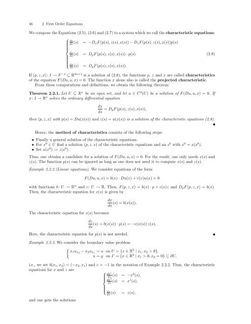
46 2 First Order Equations
We compose the Equations (2.5), (2.6) and (2.7) to a system which we call the characteristic equations:
⎧
dp
ds (s) = −D xF (p(s), z(s), x(s)) − D z F (p(s), z(s), x(s))p(s)
⎪⎨
= D pF (p(s), z(s), x(s)) · p(s)
(2.8)
dz
ds (s)
⎪⎩ dx
ds (s)
= D pF (p(s), z(s), x(s)).
If (p, z, x): I → F −1 ⊆ R 2n+1 is a solution of (2.8), the functions p, z and x are called characteristics
of the equation F (Du, u, x) = 0. The function x alone also is called the projected characteristic.
From these computations and definitions, we obtain the following theorem:
Theorem 2.2.1. Let U ⊆ R n be an open set, and let u ∈ C 2 (U) be a solution of F (Du, u, x) = 0. If
x: I → R n solves the ordinary differential equation
dx
ds = D pF (p(s), z(s), x(s)),
then (p, z, x) with p(s) = Du(x(s)) and z(s) = u(x(s)) is a solution of the characteristic equations (2.8).
Hence, the method of characteristics consists of the following steps:
• Finally a general solution of the characteristic equations.
• For x 0 ∈ U find a solution (p, z, x) of the characteristic equations and an s 0 with x 0 = x(s 0 ).
• Set u(x 0 ) := z(s 0 ).
Thus, one obtains a candidate for a solution of F (Du, u, x) = 0. For the result, one only needs x(s) and
z(s). The function p(s) can be ignored as long as one does not need it to compute x(s) and z(s).
Example 2.2.2 (Linear equations). We consider equations of the form
F (Du, u, x) = b(x) · Du(x) + c(x)u(x) = 0
with functions b: U → R n and c: U → R. Then, F (p, z, x) = b(x) · p + c(x)z and D p F (p, z, x) = b(x).
Then, the characteristic equation for x(s) is given by
The characteristic equation for z(s) becomes
dx
(s) = b(x(s)).
ds
dz
(s) = b(x(s)) · p(s) = −c(x(s)) z(s).
ds
Here, the characteristic equation for p(s) is not needed.
Example 2.2.3. We consider the boundary value problem
{
x1 u x2 − x 2 u x1 = u on U = {x ∈ R 2 | x 1 , x 2 > 0},
u = g on Γ = {x ∈ R 2 | x 1 > 0, x 2 = 0} ⊆ ∂U,
i.e., we set b(x 1 , x 2 ) = (−x 2 , x 1 ) and c = −1 in the notation of Example 2.2.2. Thus, the characteristic
equations for x and z are
⎧
dx 1
ds
⎪⎨
(s) = −x2 (s),
dx 2
ds (s) = x1 (s),
and one gets the solutions
⎪⎩ dz
ds (s)
= z(s),