Partial Differential Equations

1.2 The Laplace Equation 7
Proof. Idea: Integrate in polar coordinates
Integration in polar coordinates shows that it suffices to prove the convergence of the integrals
∫ R
0
(log r)r dr
and
∫ R
0
1
r n−2 rn−1 dr.
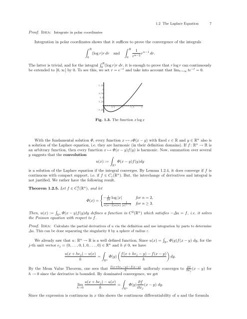
The latter is trivial, and for the integral ∫ R
(log r)r dr, it is enough to prove that r log r can continuously
0
be extended to [0, ∞[ by 0. To see this, we set r = e −t and take into account that lim t→∞ te −t = 0.
1.25
1
0.75
0.5
0.25
-0.25
0.5 1 1.5 2
Fig. 1.3. The function x log x
With the fundamental solution Φ, every function x ↦→ cΦ(x − y) with fixed c ∈ R and y ∈ R n also is
a solution of the Laplace equation, i.e. they are harmonic (in their definition domains). If f : R n → R is
an arbitrary function, then every function x ↦→ Φ(x − y)f(y) is harmonic. Now, summation over several
y suggests that the convolution
∫
u(x) := Φ(x − y)f(y)dy
R n
is a solution of the Laplace equation if the integral converges. By Lemma 1.2.4, it does converge if f is
continuous with compact support, i.e. if f ∈ C c (R n ). But, the interchange of derivatives and integral is
not justified. We rather have the following result.
Theorem 1.2.5. Let f ∈ Cc 2 (R n ), and let
{
−
1
2π
log |x| for n = 2,
Φ(x) =
1 1
n(n−2)α(n) |x|
for n ≥ 3.
n−2
Then, u(x) := ∫ R n Φ(x − y)f(y)dy defines a function in C 2 (R n ) which satisfies −∆u = f, i.e. it solves
the Poisson equation with respect to f.
Proof. Idea: Calculate the partial derivatives of u via the definition and use integration by parts to determine
∆u. This can be done separating the singularity 0 by a sphere of radius ε.
We already saw that u: R n → R is a well defined function. Since u(x) = ∫ Φ(y)f(x − y) dy, for the
R n
j-th unit vector e j = (0, . . . , 0, 1, 0, . . . , 0) ∈ R n and h ≠ 0, we have
∫ ( )
u(x + he j ) − u(x)
f(x + hej − y) − f(x − y)
= Φ(y)
dy.
h
R h
n
By the Mean Value Theorem, one sees that f(x+hej−y)−f(x−y)
h
uniformly converges to ∂f
∂x j
(x − y) for
h → 0 since the derivative is bounded. By dominated convergence, we get
u(x + he j ) − u(x)
lim
=
h→0 h
∫
R n Φ(y) ∂f
∂x j
(x − y) dy.
Since the expression is continuous in x this shows the continuous differentiability of u and the formula