Partial Differential Equations
Partial Differential Equations
Partial Differential Equations

You also want an ePaper? Increase the reach of your titles
YUMPU automatically turns print PDFs into web optimized ePapers that Google loves.
<strong>Partial</strong> <strong>Differential</strong> <strong>Equations</strong><br />
Summer Term 2009<br />
Joachim Hilgert<br />
This is a preliminary set of notes and not meant for general distribution. It is not proofread.<br />
Paderborn, July 20, 2009<br />
J. Hilgert
Contents<br />
1 The Fundamental <strong>Partial</strong> <strong>Differential</strong> <strong>Equations</strong> . . . . . . . . . . . . . . . . . . . . . . . . . . . . . . . . . . 3<br />
1.1 The Transport Equation . . . . . . . . . . . . . . . . . . . . . . . . . . . . . . . . . . . . . . . . . . . . . . . . . . . . . . . . . 3<br />
1.2 The Laplace Equation . . . . . . . . . . . . . . . . . . . . . . . . . . . . . . . . . . . . . . . . . . . . . . . . . . . . . . . . . . . 5<br />
1.3 The Heat Equation . . . . . . . . . . . . . . . . . . . . . . . . . . . . . . . . . . . . . . . . . . . . . . . . . . . . . . . . . . . . . 18<br />
1.4 The Wave Equation. . . . . . . . . . . . . . . . . . . . . . . . . . . . . . . . . . . . . . . . . . . . . . . . . . . . . . . . . . . . . 25<br />
2 First Order <strong>Equations</strong> . . . . . . . . . . . . . . . . . . . . . . . . . . . . . . . . . . . . . . . . . . . . . . . . . . . . . . . . . . . 41<br />
2.1 Complete Integrals and Enveloping Functions . . . . . . . . . . . . . . . . . . . . . . . . . . . . . . . . . . . . . . 41<br />
2.2 The Method of Characteristics . . . . . . . . . . . . . . . . . . . . . . . . . . . . . . . . . . . . . . . . . . . . . . . . . . . 45<br />
2.3 Local Existence of Solutions . . . . . . . . . . . . . . . . . . . . . . . . . . . . . . . . . . . . . . . . . . . . . . . . . . . . . 52<br />
2.4 Hamilton–Jacobi <strong>Equations</strong> . . . . . . . . . . . . . . . . . . . . . . . . . . . . . . . . . . . . . . . . . . . . . . . . . . . . . . 57<br />
3 Various Solution Techniques . . . . . . . . . . . . . . . . . . . . . . . . . . . . . . . . . . . . . . . . . . . . . . . . . . . . . . 65<br />
3.1 Separation of Variables . . . . . . . . . . . . . . . . . . . . . . . . . . . . . . . . . . . . . . . . . . . . . . . . . . . . . . . . . . 65<br />
3.2 Traveling Waves . . . . . . . . . . . . . . . . . . . . . . . . . . . . . . . . . . . . . . . . . . . . . . . . . . . . . . . . . . . . . . . . 67<br />
3.3 Fourier and Laplace Transformation . . . . . . . . . . . . . . . . . . . . . . . . . . . . . . . . . . . . . . . . . . . . . . 70<br />
3.4 The Theorem of Cauchy–Kovalevskaya . . . . . . . . . . . . . . . . . . . . . . . . . . . . . . . . . . . . . . . . . . . . 75<br />
3.5 The Counterexample of Lewy . . . . . . . . . . . . . . . . . . . . . . . . . . . . . . . . . . . . . . . . . . . . . . . . . . . . 82<br />
4 Linear <strong>Differential</strong> Operators with Constant Coefficients . . . . . . . . . . . . . . . . . . . . . . . . . . 85<br />
4.1 Fundamental Solutions . . . . . . . . . . . . . . . . . . . . . . . . . . . . . . . . . . . . . . . . . . . . . . . . . . . . . . . . . . 85<br />
4.2 Elliptic Regularity . . . . . . . . . . . . . . . . . . . . . . . . . . . . . . . . . . . . . . . . . . . . . . . . . . . . . . . . . . . . . . 90<br />
A Function Spaces . . . . . . . . . . . . . . . . . . . . . . . . . . . . . . . . . . . . . . . . . . . . . . . . . . . . . . . . . . . . . . . . . . 93<br />
A.1 L p –spaces . . . . . . . . . . . . . . . . . . . . . . . . . . . . . . . . . . . . . . . . . . . . . . . . . . . . . . . . . . . . . . . . . . . . . 93<br />
A.2 Topological Vector Spaces . . . . . . . . . . . . . . . . . . . . . . . . . . . . . . . . . . . . . . . . . . . . . . . . . . . . . . . 102<br />
A.3 Spaces of Differentiable Functions . . . . . . . . . . . . . . . . . . . . . . . . . . . . . . . . . . . . . . . . . . . . . . . . 107<br />
A.4 The Fourier Transform . . . . . . . . . . . . . . . . . . . . . . . . . . . . . . . . . . . . . . . . . . . . . . . . . . . . . . . . . . 112<br />
B Distributions . . . . . . . . . . . . . . . . . . . . . . . . . . . . . . . . . . . . . . . . . . . . . . . . . . . . . . . . . . . . . . . . . . . . . 117<br />
B.1 Tempered Distributions . . . . . . . . . . . . . . . . . . . . . . . . . . . . . . . . . . . . . . . . . . . . . . . . . . . . . . . . . 117<br />
B.2 Distributions . . . . . . . . . . . . . . . . . . . . . . . . . . . . . . . . . . . . . . . . . . . . . . . . . . . . . . . . . . . . . . . . . . . 122<br />
B.3 Convergence of Distributions . . . . . . . . . . . . . . . . . . . . . . . . . . . . . . . . . . . . . . . . . . . . . . . . . . . . . 130<br />
C Sobolev spaces . . . . . . . . . . . . . . . . . . . . . . . . . . . . . . . . . . . . . . . . . . . . . . . . . . . . . . . . . . . . . . . . . . . . 133<br />
C.1 General theory . . . . . . . . . . . . . . . . . . . . . . . . . . . . . . . . . . . . . . . . . . . . . . . . . . . . . . . . . . . . . . . . . 133<br />
C.2 Localised Sobolev spaces . . . . . . . . . . . . . . . . . . . . . . . . . . . . . . . . . . . . . . . . . . . . . . . . . . . . . . . . 140<br />
C.3 Boundary values . . . . . . . . . . . . . . . . . . . . . . . . . . . . . . . . . . . . . . . . . . . . . . . . . . . . . . . . . . . . . . . 146<br />
C.4 Difference quotients . . . . . . . . . . . . . . . . . . . . . . . . . . . . . . . . . . . . . . . . . . . . . . . . . . . . . . . . . . . . . 148<br />
Index . . . . . . . . . . . . . . . . . . . . . . . . . . . . . . . . . . . . . . . . . . . . . . . . . . . . . . . . . . . . . . . . . . . . . . . . . . . . . . . . . 151
Preface<br />
Let U ⊆ R n be an open set and u = (u 1 , . . . , u m ): U → R m a k–times differentiable function. Then<br />
the gradient map<br />
Du: U → Mat(m × n, R) ∼ = R mn<br />
⎛<br />
⎞<br />
∂u 1 (x)<br />
∂x 1<br />
. . .<br />
x ↦→ ⎜<br />
⎝<br />
.<br />
∂u m (x)<br />
∂x 1<br />
∂u 1 (x)<br />
∂x n<br />
.<br />
. . . ∂um (x)<br />
∂x n<br />
is (k − 1)–times differentiable and one can repeat the procedure until one finds a map<br />
D k u: U → R mnk .<br />
⎟<br />
⎠<br />
A partial differential equation is an equation of the form<br />
F (D k u(x), D k−1 u(x), . . . , Du(x), u(x), x) = 0,<br />
where F : R nk × R nk−1 × . . . × R n × R × U → R is a given function and u: U → R is the function one<br />
wants to determine.<br />
A system of partial differential equations is an equation of the form<br />
F (D k u(x), D k−1 u(x), . . . , Du(x), u(x), x) = 0,<br />
where F : R mnk × R mnk−1 × . . . × R mn × R m × U → R l is a given function and u: U → R m is the function<br />
one wants to determine.
1<br />
The Fundamental <strong>Partial</strong> <strong>Differential</strong> <strong>Equations</strong><br />
In the theory of partial differentiable equations, a number of notations and abbreviations became<br />
established which have the intension to make the often intricate formulas more transparent. For instance,<br />
one often abbreviates ∂u<br />
∂x by u ∂<br />
x, or 2 u<br />
∂x∂y<br />
by u xy. In many examples, time appears as variable t with<br />
separate meaning. In such cases, the notation Du often only refers to the other variables.<br />
1.1 The Transport Equation<br />
The (homogeneous) transport equation is the partial differential equation<br />
u t + b · Du = 0,<br />
where u: R n × ]0, ∞[ → R is the unknown function, b ∈ R n is a fixed vector, and Du(·, t): R n → R n is<br />
the gradient map with respect to the variables in R n . Further, b · Du(x, t) ∈ R is the Euclidean scalar<br />
product of b and Du(x, t).<br />
To solve the transport equation, one first fixes a point (x, t) ∈ R n × ]0, ∞[ and supposes that one<br />
has a differentiable solution u: R n × ]0, ∞[ −→ R which can be extended to a continuous function on<br />
R n × [0, ∞[. The function z : ] − t, ∞[→ R which is defined by<br />
then satisfies the ordinary differential equation<br />
ż(s) := dz(s)<br />
ds<br />
z(s) := u(x + sb, t + s)<br />
= Du(x + sb, t + s) · b + u t (x + sb, t + s) = 0<br />
by the chain rule.<br />
Thus, z is constant which in turn shows that the solution u is constant on the half-lines {(x, t)+s(b, 1) ⊆<br />
R n × ]0, ∞[}.<br />
We consider the initial value problem which corresponds to the transport equation<br />
{<br />
ut + b · Du = 0 on R n × ]0, ∞[,<br />
u = g on R n (1.1)<br />
× {0},<br />
where g : R n → R is a known function, and where u: R n × R + → R is a continuous unknown function.<br />
As before, one sees that the function u is constant for every x ∈ R n on the half-line (x, 0)+ ]0, ∞[ (b, 1).<br />
The continuous extension onto R n × [0, ∞[ then shows that u(x + sb, s) = g(x) or, with other words,<br />
u(x, t) = g(x − tb). (1.2)
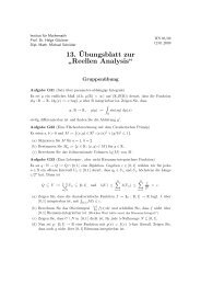
4 1 The Fundamental <strong>Partial</strong> <strong>Differential</strong> <strong>Equations</strong><br />
(x,t)+ R(b,1)<br />
t<br />
(x,t)<br />
x<br />
x+ R b<br />
Fig. 1.1. Transport equation<br />
Hence, if there is a continuous solution of the initial problem, then it is of the form (x, t) ↦→ g(x − tb).<br />
Then, g has to be differentiable. Conversely, if g is differentiable, then u(x, t) = g(x − tb) indeed defines<br />
a continuous solution of the problem.<br />
We consider the following inhomogeneous initial value problem which corresponds to the transport<br />
equation<br />
{<br />
ut + b · Du = f on R n × ]0, ∞[,<br />
u = g on R n (1.3)<br />
× {0},<br />
where g : R n → R and f : R n ×]0, ∞[ now are two known (continuous) functions, and u: R n × R + → R is<br />
the continuous unknown function.<br />
Here, the solution strategy via ordinary differential equations can also be employed: For fixed (x, t) ∈<br />
R n ×]0, ∞[ and a differentiable solution u: R n ×]0, ∞[→ R, one again sets z(s) := u(x + sb, t + s). This<br />
time, the ordinary differential equation<br />
ż(s) := dz(s)<br />
ds<br />
is obtained. It is solved by<br />
Now, we get<br />
= Du(x + sb, t + s) · b + u t (x + sb, t + s) = f(x + sb, t + s)<br />
z(s) = z(0) +<br />
∫ s<br />
u(x + sb, t + s) − u(x, t) =<br />
0<br />
f(x + σb, t + σ)dσ.<br />
∫ s<br />
0<br />
f(x + σb, t + σ)dσ<br />
and the continuity of u gives for s = −t that<br />
∫ 0<br />
u(x, t) = g(x − tb) + f(x + σb, t + σ)dσ = g(x − tb) +<br />
−t<br />
∫ t<br />
0<br />
f(x + (σ − t)b, σ)dσ. (1.4)<br />
By the uniqueness assertion in the Picard–Lindelöf Theorem, we now obtain the following proposition.<br />
Proposition 1.1.1. Let g ∈ C 1 (R n ) and b ∈ R n . Then, the initial value problem (1.3) has a uniquely<br />
determined C 1 -solution u: R n × ]0, ∞[ → R which is continuously extendable onto R n × [0, ∞[, and which<br />
is given by Formula (1.4).<br />
Proof. It only remains to show uniqueness. This follows from the unique solvability of the involved<br />
ordinary differential equations.<br />
The transport equation is a special case of the Boltzmann transport equation which describes the timedependent<br />
behavior of a thin gas in phase space [cf. J.R. Dorfman und H. Van Beijeren, “The Kinetic<br />
Theory of Gases”in Statistical Mechanics, Part B, B. Berne ed., Plenum Press, New York (1976)]. There,<br />
the homogeneous case with constant b just describes the time-dependent expansion of a gas in which all<br />
particles have the same velocity b and no impact processes appear between particles. Impact processes<br />
then give an inhomogeneity.
1.2 The Laplace Equation 5<br />
Fig. 1.2. Transport equation<br />
Exercise 1.1.2. Provide an explicit solution of the following initial value problem:<br />
{<br />
ut + b · Du + cu = 0 on R n × ]0, ∞[,<br />
u = g on R n × {0}.<br />
Here, c ∈ R and b ∈ R n are constants.<br />
1.2 The Laplace Equation<br />
The Laplace equation is the partial differential equation<br />
∆u = 0,<br />
where u: R n → R and ∆u = ∑ n<br />
j=1 ∂2 u<br />
∂x j<br />
2 . The solutions of the Laplace equation are called harmonic<br />
functions. The inhomogeneous version<br />
−∆u = f<br />
of the Laplace equation, where f : R n → R is a given function, and again u: R n → R is the unknown<br />
function, is also called Poisson equation.<br />
The Laplace equation describes an equilibrium state of densities u whose flux F is described by<br />
F = −aDu. By the divergence theorem, equilibrium then means that<br />
∫ ∫<br />
div F = F · ν dS ∂V = 0,<br />
V<br />
hence, div F = 0 (with infinitesimal V ), and therefore, ∆u = div Du = − 1 adiv F = 0.<br />
∂V<br />
First, we look for radial solutions of the Laplace, i.e. solutions u of the form u(x) = v(r), where<br />
r = √ x 2 1 + . . . + x2 n is the Euclidean norm |x| of x. Because of<br />
for x ≠ 0, we have, for radial u, that<br />
∂r x<br />
= √ j<br />
= x j<br />
∂x j x<br />
2<br />
1 + . . . + x 2 r<br />
n<br />
u xj (x) = v ′ (r) x j<br />
r ,<br />
u xjx j<br />
(x) = v ′′ (r) x2 j<br />
r 2 + v′ (r) 1 r<br />
(<br />
1 − x2 j<br />
r 2 )<br />
for all j = 1, . . . , n, and thus,<br />
∆u(x) = v ′′ (r) + n − 1 v ′ (r).<br />
r<br />
Therefore, ∆u = 0 is equivalent to the ordinary differential equation
6 1 The Fundamental <strong>Partial</strong> <strong>Differential</strong> <strong>Equations</strong><br />
v ′′ (r) + n − 1 v ′ (r) = 0. (1.5)<br />
r<br />
To get a solution of (1.5), we first assume that we have a solution with v ′ (r) > 0 for all r. Then,<br />
log(v ′ ) ′ (r) = v′′ (r)<br />
v ′ (r) = 1 − n ,<br />
r<br />
and hence, log v ′ (r) = (1 − n) log r + a. This, we rewrite to v ′ (r) =<br />
v(r) =<br />
{<br />
b log r + c for n = 2,<br />
b<br />
r<br />
+ c n−2 for n ≥ 3,<br />
ea<br />
r n−1<br />
, and we get the solutions<br />
where b, and c, resp., are (arbitrary) constants in R + , and R, resp. For v ′ (r) < 0, one gets the same<br />
formulas with negative b.<br />
The function Φ: R n \ {0} → R which is defined by<br />
{<br />
−<br />
1<br />
2π<br />
log |x| for n = 2,<br />
Φ(x) =<br />
1 1<br />
n(n−2)α(n) |x|<br />
for n ≥ 3,<br />
n−2<br />
where<br />
α(n) = vol(B(0; 1)) = 2 n Γ ( 1 2 + 1)n<br />
Γ ( n 2 + 1) = π n 2<br />
Γ ( n 2 + 1)<br />
is the volume of the unit ball in R n , satisfies ∆Φ = 0 on R n \ {0}, and it is called the fundamental<br />
solution of the Laplace equation.<br />
Exercise 1.2.1. For n ≥ 2, show by explicit calculations that the function<br />
is harmonic for y ∈ ∂B(0; r) ⊆ R n .<br />
B(0; r) → R,<br />
x ↦→ r2 − |x| 2<br />
|y − x| n<br />
Exercise 1.2.2. Show that the Laplace equation ∆u = 0 on R n is invariant under rotations, i.e. if A is<br />
an orthogonal (n × n)-matrix, and v(x) := u(Ax), then ∆v = 0.<br />
Remark 1.2.3. The fundamental solution Φ of the Laplace equation satisfies the following estimations:<br />
where C is a constant depending on n.<br />
|DΦ(x)| ≤<br />
C<br />
|x| n−1 ,<br />
|D 2 Φ(x)| ≤ C<br />
|x| n ,<br />
We will need the following result for the construction of solutions of the Poisson equation. Note that<br />
in higher dimensions, we also denote the Lebesgue measure by dx (instead of dλ(x)).<br />
Lemma 1.2.4. The integral<br />
exists for all R > 0.<br />
∫<br />
B(0;R)<br />
Φ(x)dx
1.2 The Laplace Equation 7<br />
Proof. Idea: Integrate in polar coordinates<br />
Integration in polar coordinates shows that it suffices to prove the convergence of the integrals<br />
∫ R<br />
0<br />
(log r)r dr<br />
and<br />
∫ R<br />
0<br />
1<br />
r n−2 rn−1 dr.<br />
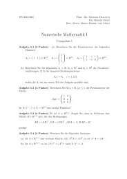
The latter is trivial, and for the integral ∫ R<br />
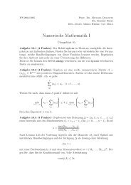
(log r)r dr, it is enough to prove that r log r can continuously<br />
0<br />
be extended to [0, ∞[ by 0. To see this, we set r = e −t and take into account that lim t→∞ te −t = 0.<br />
1.25<br />
1<br />
0.75<br />
0.5<br />
0.25<br />
-0.25<br />
0.5 1 1.5 2<br />
Fig. 1.3. The function x log x<br />
With the fundamental solution Φ, every function x ↦→ cΦ(x − y) with fixed c ∈ R and y ∈ R n also is<br />
a solution of the Laplace equation, i.e. they are harmonic (in their definition domains). If f : R n → R is<br />
an arbitrary function, then every function x ↦→ Φ(x − y)f(y) is harmonic. Now, summation over several<br />
y suggests that the convolution<br />
∫<br />
u(x) := Φ(x − y)f(y)dy<br />
R n<br />
is a solution of the Laplace equation if the integral converges. By Lemma 1.2.4, it does converge if f is<br />
continuous with compact support, i.e. if f ∈ C c (R n ). But, the interchange of derivatives and integral is<br />
not justified. We rather have the following result.<br />
Theorem 1.2.5. Let f ∈ Cc 2 (R n ), and let<br />
{<br />
−<br />
1<br />
2π<br />
log |x| for n = 2,<br />
Φ(x) =<br />
1 1<br />
n(n−2)α(n) |x|<br />
for n ≥ 3.<br />
n−2<br />
Then, u(x) := ∫ R n Φ(x − y)f(y)dy defines a function in C 2 (R n ) which satisfies −∆u = f, i.e. it solves<br />
the Poisson equation with respect to f.<br />
Proof. Idea: Calculate the partial derivatives of u via the definition and use integration by parts to determine<br />
∆u. This can be done separating the singularity 0 by a sphere of radius ε.<br />
We already saw that u: R n → R is a well defined function. Since u(x) = ∫ Φ(y)f(x − y) dy, for the<br />
R n<br />
j-th unit vector e j = (0, . . . , 0, 1, 0, . . . , 0) ∈ R n and h ≠ 0, we have<br />
∫ ( )<br />
u(x + he j ) − u(x)<br />
f(x + hej − y) − f(x − y)<br />
= Φ(y)<br />
dy.<br />
h<br />
R h<br />
n<br />
By the Mean Value Theorem, one sees that f(x+hej−y)−f(x−y)<br />
h<br />
uniformly converges to ∂f<br />
∂x j<br />
(x − y) for<br />
h → 0 since the derivative is bounded. By dominated convergence, we get<br />
u(x + he j ) − u(x)<br />
lim<br />
=<br />
h→0 h<br />
∫<br />
R n Φ(y) ∂f<br />
∂x j<br />
(x − y) dy.<br />
Since the expression is continuous in x this shows the continuous differentiability of u and the formula
8 1 The Fundamental <strong>Partial</strong> <strong>Differential</strong> <strong>Equations</strong><br />
∫<br />
∂u<br />
(x) = Φ(y) ∂f (x − y) dy.<br />
∂x j R ∂x n j<br />
With the same argument, we obtain that u is twice differentiable, and we get the formula<br />
∂ 2 ∫<br />
u<br />
∂ 2 f<br />
(x) = Φ(y) (x − y) dy.<br />
∂x i ∂x j R ∂x n i ∂x j<br />
The right hand side of this formula again is continuous in x, hence, u ∈ C 2 (R n ).<br />
To compute ∆u, we split the integral into<br />
∫<br />
∫<br />
∆u = Φ(y)∆ x f(x − y) dy<br />
Φ(y)∆ x f(x − y) dy<br />
B(0;ε)<br />
} {{ }<br />
I ε<br />
+<br />
R n \B(0;ε)<br />
} {{ }<br />
J ε<br />
,<br />
where ∆ x is the corresponding derivative with respect to the x-variable. Let<br />
{∣ ∣∣∣<br />
‖D 2 ∂ 2 }<br />
f<br />
f‖ ∞ := sup (x)<br />
∂x i ∂x j<br />
∣ : x ∈ Rn ; i, j = 1, . . . , n .<br />
Then,<br />
|I ε | ≤ n‖D 2 f‖ ∞<br />
∫<br />
B(0;ε)<br />
|Φ(y)| dy ≤<br />
{<br />
Cε 2 | log ε| for n = 2,<br />
Cε 2 for n ≥ 3,<br />
where the radial integrals in the proof of Lemma 1.2.4 are estimated for small ε > 0 (such that ε log ε is<br />
monotonic). Gauß’ Integral Theorem<br />
∫<br />
∫<br />
div F (x) dx = F (x) · ν(x) dS ∂A (x),<br />
A<br />
∂A<br />
applied to a vector field of the form F (x) = (0, . . . , 0, uv, 0, . . . , 0) (uv at j-th position), gives the following<br />
integration by parts formula<br />
∫<br />
∫<br />
∫<br />
u xj (x)v(x)dx = − u(x)v xj (x)dx + u(x)v(x)ν(x) j dS ∂A (x), (1.6)<br />
A<br />
A<br />
∂A<br />
where ν(x) j denotes the j-th component of the normal vector ν(x). If v = w xj , then this formula leads<br />
to<br />
∫<br />
∫<br />
∫<br />
∂w<br />
Du(x) · Dw(x)dx = − u(x)∆w(x)dx +<br />
∂ν (x)u(x) dS ∂A(x) (1.7)<br />
(sum over j = 1, . . . , n), where<br />
A<br />
∂w<br />
∂ν (a) := (w′ (a))(ν(a)) =<br />
n∑<br />
j=1<br />
A<br />
∂A<br />
∂w<br />
∂x j<br />
(a)ν j (a) = (grad w(a) | ν(a)) = Dw(a) · ν(a). (1.8)<br />
Now, we choose a spherical shell whose inner boundary is ∂B(0; ε), and f together with its derivatives<br />
vanish on its outer boundary. Then, we calculate<br />
∫<br />
J ε = Φ(y)∆ y f(x − y) dy<br />
∫<br />
= −<br />
R n \B(0;ε)<br />
R n \B(0;ε)<br />
DΦ(y) · D y f(x − y) dy<br />
} {{ }<br />
K ε<br />
+<br />
∫<br />
Φ(y) ∂f<br />
∂B(0;ε) ∂ν (x − y) dS ∂B(0;ε)(y)<br />
} {{ }<br />
L ε<br />
.<br />
With<br />
{∣ }<br />
∣∣∣ ∂f<br />
‖Df‖ ∞ := sup (x)<br />
∂x j<br />
∣ : x ∈ Rn ; j = 1, . . . , n ,
we obtain the estimate<br />
|L ε | ≤ n‖Df‖ ∞<br />
∫<br />
∂B(0;ε)<br />
|Φ(y)| dS ∂B(0;ε) (y) ≤<br />
Applying integration by parts again, we find<br />
∫<br />
∫<br />
K ε = ∆ y Φ(y)f(x − y) dy −<br />
∫<br />
= −<br />
R n \B(0;ε)<br />
∂B(0;ε)<br />
∂B(0;ε)<br />
∂Φ<br />
∂ν (y)f(x − y) dS ∂B(0;ε)(y)<br />
1.2 The Laplace Equation 9<br />
{<br />
Cε| log ε| for n = 2,<br />
Cε for n ≥ 3.<br />
∂Φ<br />
∂ν (y)f(x − y) dS ∂B(0;ε)(y)<br />
since Φ is harmonic in R n \ {0}. Note that ν(y) = y ε<br />
for y ∈ ∂B(0; ε). Moreover, we have<br />
0<br />
ε<br />
y<br />
1<br />
Fig. 1.4.<br />
From this, for n ≥ 3, we obtain<br />
DΦ(y) =<br />
{<br />
−<br />
1<br />
2π<br />
y<br />
− 1<br />
nα(n)<br />
|y| 2 ∀y ≠ 0 if n = 2<br />
y<br />
|y| n ∀y ≠ 0 if n ≥ 3.<br />
∂Φ<br />
∂ν (y) = ν(y) · DΦ(y) = − 1<br />
nα(n)ε n−1<br />
∀y ∈ ∂B(0; ε).<br />
The surface area of ∂B(0; ε) is nα(n)ε n−1 . Now, the continuity of f in x gives<br />
K ε = −<br />
1<br />
nα(n)ε n−1 ∫∂B(0;ε)<br />
f(x − y) dS ∂B(0;ε) (y) −→<br />
ε→0<br />
−f(x).<br />
Similarly we find K ε −→<br />
ε→0<br />
−f(x) also for n = 2. Together with the already proven estimations for L ε and<br />
I ε , we finally conclude<br />
∆u(x) = lim<br />
ε→0<br />
(I ε + L ε + K ε ) = −f(x).<br />
Let U ⊆ R n be open and bounded with smooth boundary ∂U. We consider the boundary value<br />
problem which corresponds to the Poisson equation:<br />
{ −∆u = f on U,<br />
(1.9)<br />
u = g on ∂U,<br />
where now f : U → R and g : ∂U → R are given, and u: U × R + → R is the unknown function (U is the<br />
closure of U in R n ).<br />
For an open subset U of R n , let C k (U) be the space of all functions u: U → R whose restriction onto<br />
U lies in C k (U) and whose partial derivatives up to order k are all uniformly continuous on U (thus, they<br />
can be extended onto U).
10 1 The Fundamental <strong>Partial</strong> <strong>Differential</strong> <strong>Equations</strong><br />
Proposition 1.2.6. Let U ⊆ R n be open and bounded with smooth boundary. Then, there is at most one<br />
solution u ∈ C 2 (U) for the boundary value problem (1.9).<br />
Proof. Idea: Integration by parts.<br />
Let u and ũ be two such solutions, and let w := u − ũ. Since ∆w = 0 on U, and since w = 0 on ∂U,<br />
integration by parts gives (cf. Formula (1.7))<br />
∫<br />
∫<br />
0 = − w(x)∆w(x) dx = |Dw(x)| 2 dx,<br />
U<br />
and the continuity of Dw shows that Dw = 0 on U. Again by w = 0 on ∂U, one concludes that w = 0<br />
on U.<br />
Later, we will see that it suffices to require u ∈ C 2 (U) for f = 0.<br />
U<br />
Lemma 1.2.7. Let u ∈ C 2 (R n ) be harmonic. Then, for all x ∈ R n and all r > 0, we have<br />
∫<br />
∫<br />
1<br />
1<br />
u(x) =<br />
vol B(x;r)<br />
u(y)dy =<br />
vol ∂B(x;r)<br />
u(y) dS ∂B(x;r) (y).<br />
B(x;r)<br />
∂B(x;r)<br />
Proof. Idea:<br />
coordinates.<br />
Apply formula (1.7) to the right hand side, viewed as a function of r. then integrate in polar<br />
Then,<br />
We set<br />
ϕ(r) :=<br />
1<br />
vol ∂B(x;r)<br />
and formula (1.7) gives<br />
∫<br />
∂B(x;r)<br />
Thus, ϕ is constant, and we have<br />
∫<br />
1<br />
u(y) dS ∂B(x;r) (y) =<br />
vol ∂B(0;1)<br />
u(x + ry) dS ∂B(0;1) (y).<br />
∂B(0;1)<br />
∫<br />
ϕ ′ 1<br />
(r) =<br />
vol ∂B(0;1)<br />
Du(x + ry) · y dS ∂B(0;1) (y),<br />
∂B(0;1)<br />
∫<br />
ϕ ′ 1<br />
(r) =<br />
vol ∂B(x;r)<br />
∫<br />
=<br />
1<br />
vol ∂B(x;r)<br />
=<br />
1<br />
vol ∂B(x;r)<br />
= 0.<br />
∫<br />
∂B(x;r)<br />
∂B(x;r)<br />
B(x;r)<br />
ϕ(r) = lim<br />
t→0<br />
ϕ(t) = lim<br />
t→0<br />
1<br />
vol ∂B(x;t)<br />
Finally, integration in polar coordinates also gives<br />
∫<br />
∫ r ∫<br />
u(y)dy =<br />
B(x;r)<br />
0<br />
= u(x)<br />
Du(y) · y − x<br />
r<br />
∂u<br />
∂ν (y) dS ∂B(x;r)(y)<br />
∆u(y)dy<br />
∫<br />
∂B(x;t)<br />
∂B(x;s)<br />
∫ r ∫<br />
0<br />
dS ∂B(x;r) (y)<br />
u(y) dS ∂B(x;t) (y) = u(x).<br />
u(y) dS ∂B(x;s) (y) ds<br />
∂B(x;s)<br />
= vol(B(x; r)) u(x).<br />
dS ∂B(x;s) (y) ds<br />
The result of Lemma 1.2.7 is also called the mean value property of harmonic functions.
1.2 The Laplace Equation 11<br />
Exercise 1.2.8. Vary the proof of the mean value property for harmonic functions to show that, for<br />
n ≥ 3, a solution of the boundary value problem<br />
{ −∆u = f on B(0; r),<br />
satisfies the integral formula<br />
∫<br />
u(0) =<br />
r n<br />
vol ∂B(0;r)<br />
∂B(0;r)<br />
u = g on ∂B(0; r)<br />
g(y) dS ∂B(0;r) (y) + 1<br />
1<br />
n(n−2) vol B(0;r)<br />
∫<br />
B(0;r)<br />
( 1<br />
|y| n−2 − 1 r 2 )<br />
f(y)dy.<br />
Theorem 1.2.9 (Maximum principle). Let U ⊆ R n be open and bounded. For every harmonic function<br />
u: U → R which can be extended continuously to U, we have<br />
(i) max x∈U<br />
u(x) = max x∈∂U u(x).<br />
(ii) Let U be connected, and let x 0 ∈ U with u(x 0 ) = max x∈U<br />
u(x), then u is constant on U.<br />
Proof. Idea: Use the mean value property to prove (ii). Then (i) follows.<br />
Since U is compact, the maxima exist, and (i) follows from (ii). To show (ii), we set M := u(x 0 ). If<br />
x ∈ U and u(x) = M, then we choose a ball B(x; r) whose closure is contained in U. Then, Lemma 1.2.7<br />
gives<br />
∫<br />
1<br />
M =<br />
u(y)dy ≤ M,<br />
vol B(x; r) B(x;r)<br />
and we have u(y) = M for all y ∈ B(x; r). Thus, u −1 (M) ⊆ U is open. But, u −1 (M) also is closed since<br />
u is continuous. Since U is assumed to be connected and u −1 (M) is nonempty, u has to be constant and<br />
equal to M.<br />
Corollary 1.2.10. Let U ⊆ R n be open and bounded. If two harmonic functions can be continuously<br />
extended onto U, and if they coincide on ∂U, then they are equal.<br />
Proof. This immediately follows from the Maximum Principle 1.2.9 for harmonic functions.<br />
Let U ⊆ R n be open and bounded. Then, by Corollary 1.2.10, there is at most one harmonic function<br />
ϕ x on U for x ∈ U which can continuously be extended onto U, and which satisfies<br />
ϕ x (y) = Φ(y − x)<br />
∀y ∈ ∂U.<br />
In case that all ϕ x exist (one can prove the existence of the ϕ x , but one needs methods which are not at<br />
our disposal yet), the function<br />
G: {(x, y) ∈ U × U | x ≠ y} → R,<br />
(x, y) ↦→ Φ(y − x) − ϕ x (y)<br />
is called Green’s function for the Laplace equation on U. Quite general, the name Green’s function is<br />
used for arbitrary open subsets U ⊆ R n as soon as one has chosen a family (ϕ x ) x∈U of harmonic functions<br />
with ϕ x (y) = Φ(x − y) for y ∈ ∂U.<br />
Lemma 1.2.11. Let U ⊆ R n be an open and bounded subset with smooth boundary. For u ∈ C 2 (U) and<br />
x ∈ U, we have the formula<br />
∫ (<br />
u(x) = − u(y) ∂Φ<br />
)<br />
∫<br />
(y − x) − Φ(y − x)∂u<br />
∂U ∂ν ∂ν (y) dS ∂U (y) − Φ(y − x)∆u(y) dy.<br />
U
12 1 The Fundamental <strong>Partial</strong> <strong>Differential</strong> <strong>Equations</strong><br />
U<br />
ν<br />
B(x; ε)<br />
ν<br />
V ε<br />
Fig. 1.5.<br />
Proof. Idea: Cut out little balls around x and apply Green’s formula to the resulting domain. The claim then<br />
follows by letting the balls shrink to x.<br />
For x ∈ U, we choose an ε > 0 with B(x; ε) ⊆ U, and we set V ε := U \ B(x; ε). Because of ∆Φ = 0 on<br />
R n \ {0}, Green’s formula<br />
∫ ∫ (<br />
(f∆g − g∆f) dλ n = f ∂g<br />
A<br />
∂A ∂ν − g ∂f )<br />
dS ∂A<br />
∂ν<br />
applied to V ε with u(y) and Φ(y − x), implies that<br />
∫<br />
(<br />
− Φ(y − x)∆u(y) dy = u(y) ∆Φ(y − x)<br />
V ε<br />
∫V ε<br />
} {{ }<br />
=0 for x≠y<br />
Moreover, we have<br />
∫<br />
∣<br />
∂B(x;ε)<br />
=<br />
∫∂V ε<br />
(<br />
)<br />
−Φ(y − x)∆u(y) dy<br />
u(y) ∂Φ<br />
)<br />
(y − x) − Φ(y − x)∂u<br />
∂ν ∂ν (y)<br />
dS ∂Vε (y).<br />
Φ(y − x) ∂u<br />
∂ν (y) dS ∂B(x;ε)(y)<br />
∣ ≤ Cεn−1 max y∈∂B(0;ε) |Φ(y)| −→<br />
ε→0<br />
0<br />
(for n > 2, this immediately follows from the formula for Φ; for n = 2, this is a consequence of<br />
lim ε→0 ε log ε = 0). The computations in the proof of Theorem 1.2.5 (more precisely, the computation for<br />
the limit of K ε ) give<br />
∫<br />
∂Φ<br />
∂ν (y − x)u(y) dS 1<br />
∂B(x;ε)(y) = −<br />
u(y) dS ∂B(x;ε) (y) −→ −u(x),<br />
ε→0<br />
∂B(x;ε)<br />
nα(n)ε n−1 ∫∂B(x;ε)<br />
hence, because of<br />
∫<br />
∫<br />
lim Φ(y − x)∆u(y) dy = Φ(y − x)∆u(y) dy<br />
ε→0<br />
V ε U<br />
(cf. Lemma 1.2.4 and the estimate of the integral I ε in the proof of Theorem 1.2.5) and ∂V ε = ∂B(x; ε) ∪<br />
∂U, we get the desired identity (note the orientation of the normal vectors!)<br />
u(x) = − lim<br />
ε→0<br />
∫∂B(x;ε)<br />
= − lim<br />
ε→0<br />
∫∂B(x;ε)<br />
= lim<br />
ε→0<br />
∫<br />
∫<br />
−<br />
∫<br />
= −<br />
∫<br />
= −<br />
∂U<br />
∂U<br />
∂U<br />
( ∂Φ<br />
∂V ε<br />
∂ν<br />
( ∂Φ<br />
∂ν<br />
( ∂Φ<br />
(<br />
∂Φ<br />
∂ν (y − x)u(y) dS ∂B(x;ε)(y)<br />
( )<br />
∂Φ<br />
(y − x)u(y) − Φ(y − x)∂u<br />
∂ν ∂ν (y)<br />
)<br />
(y − x)u(y) − Φ(y − x)∂u<br />
∂ν (y)<br />
)<br />
(y − x)u(y) − Φ(y − x)∂u<br />
∂ν (y)<br />
)<br />
(y − x)u(y) − Φ(y − x)∂u<br />
∂ν ∂ν (y)<br />
u(y) ∂Φ<br />
)<br />
(y − x) − Φ(y − x)∂u<br />
∂ν ∂ν (y)<br />
dS ∂Vε (y)<br />
dS ∂U (y)<br />
dS ∂B(x;ε) (y)<br />
dS ∂U (y) − lim Φ(y − x)∆u(y) dy<br />
V<br />
∫<br />
ε<br />
dS ∂U (y) − Φ(y − x)∆u(y) dy.<br />
ε→0<br />
∫<br />
U
1.2 The Laplace Equation 13<br />
Lemma 1.2.12. Let U ⊆ R n be an open and bounded subset with smooth boundary. For u ∈ C 2 (U) and<br />
x ∈ U, we have the formula<br />
∫<br />
u(x) = − u(y) ∂G<br />
∫<br />
∂U ∂ν (x, y) dS ∂U(y) − G(x, y)∆u(y) dy,<br />
U<br />
where G is Green’s function for the Laplace equation on U and ∂G<br />
∂ν (x, y) := D yG(x, y) · ν(y) for y ∈ ∂U.<br />
Proof. Green’s formula gives that<br />
∫<br />
∫<br />
− ϕ x (y)∆u(y) dy =<br />
U<br />
∫<br />
=<br />
∂U<br />
∂U<br />
(u(y) ∂ϕx<br />
∂ν (y) − ϕx (y) ∂u )<br />
∂ν (y) dS ∂U (y)<br />
)<br />
(u(y) ∂ϕx (y) − Φ(y − x)∂u<br />
∂ν ∂ν (y) dS ∂U (y).<br />
Adding this to the representing formula of u(x) in Lemma 1.2.11, we then obtain the claim.<br />
Theorem 1.2.13. Let U ⊆ R n be an open and bounded subset with smooth boundary, and let G be Green’s<br />
function for the Laplace equation on U. If u ∈ C 2 (U) is a solution of the boundary value problem (1.9),<br />
then for all x ∈ U, we have<br />
∫<br />
u(x) = − g(y) ∂G<br />
∫<br />
∂ν (x, y) dS ∂U(y) + G(x, y)f(y) dy.<br />
U<br />
Proof. This immediately follows by Lemma 1.2.12.<br />
∂U<br />
Example 1.2.14 (Balls). Let n ≥ 2, and let x ∈ R n \ {0}. Then, ˜x :=<br />
with respect to the inversion through the unit sphere S n−1 := ∂B(0; 1).<br />
x<br />
|x| 2<br />
is called the point dual to x<br />
x<br />
~<br />
x<br />
S n-1<br />
0<br />
Fig. 1.6.<br />
We set<br />
for x ≠ 0 and<br />
ϕ x (y) := Φ ( |x|(y − ˜x) )<br />
{<br />
0 for n = 2,<br />
ϕ 0 (y) :=<br />
1<br />
n(n−2)α(n)<br />
for n ≥ 3,<br />
i.e. ϕ 0 (y) = Φ( y<br />
|y|<br />
) for y ≠ 0. From the explicit formula<br />
{<br />
−<br />
1<br />
ϕ x 2π<br />
log |x| |y − ˜x| for n = 2,<br />
(y) =<br />
1<br />
1<br />
n(n−2)α(n) |x| n−2 |y−˜x|<br />
for n ≥ 3,<br />
n−2
14 1 The Fundamental <strong>Partial</strong> <strong>Differential</strong> <strong>Equations</strong><br />
one verifies that all ϕ x are harmonic on B(0; 1). The calculation<br />
|x| 2 |y − ˜x| 2 = |x| 2 (<br />
|y| 2 − 2y · x<br />
|x| 2 + 1<br />
|x| 2 )<br />
= |x| 2 − 2y · x + 1 = |x − y| 2<br />
for y ∈ S n−1 , we see that ϕ x (y) = Φ(y −x) for y ∈ S n−1 . If x ∈ B(0; 1), then ϕ x is defined and continuous<br />
on the entire ball B(0; 1). The function ϕ 0 is harmonic, being constant, but it also satisfies ϕ 0 (y) = Φ(y)<br />
for y ∈ S n−1 , i.e. the boundary conditions which are required in the definition of Green’s function. Thus,<br />
there is a Green’s function for B(0; 1), and it is given by<br />
{ ( )<br />
Φ(y − x) − Φ |x|(y − ˜x) for x ≠ 0,<br />
G(x, y) =<br />
Φ(y) − Φ( y<br />
|y|<br />
) for x = 0.<br />
Hence, if u ∈ C 2 (B(0; 1)) solves the initial value problem<br />
{ −∆u = 0 on B(0; 1),<br />
u = g on S n−1 ,<br />
then, we have<br />
by Theorem 1.2.13. Because of ∂Φ<br />
∂y j<br />
(y − x) = − 1<br />
and therefore,<br />
Hence, we obtain the Poisson formula<br />
∫<br />
u(x) = − g(y) ∂G<br />
S ∂ν (x, y) dS S n−1(y)<br />
n−1<br />
y j−x j<br />
nα(n) |y−x| n<br />
(check this!), for y ∈ S n−1 , we have<br />
∂G<br />
(x, y) = − 1 (<br />
yj − x j<br />
∂y j nα(n) |y − x| n − y )<br />
|x|2−n j − ˜x j<br />
|y − ˜x| n<br />
= − 1 ( )<br />
yj − x j<br />
nα(n) |y − x| n − |x|2 y j − x j<br />
|x| n |y − ˜x| n<br />
= − 1 ( )<br />
yj − x j<br />
nα(n) |y − x| n − |x|2 y j − x j<br />
|y − x| n<br />
= − 1 1 − |x| 2<br />
nα(n) |y − x| n y j,<br />
∂G<br />
1<br />
(x, y) = −<br />
∂ν nα(n)<br />
u(x) = 1 − |x|2<br />
nα(n)<br />
which can immediately be generalized to<br />
u(x) = r2 − |x| 2<br />
nα(n)r<br />
∫<br />
∫<br />
S n−1<br />
∂B(0;r)<br />
by an easy transformation of variables (here g lives on ∂B(0; r)). The function<br />
K r : B(0; r) × ∂B(0; r) → R,<br />
is also called the Poisson kernel for the ball B(0; r).<br />
1 − |x| 2<br />
|y − x| n . (1.10)<br />
g(y)<br />
|y − x| n dS Sn−1(y) (1.11)<br />
g(y)<br />
|y − x| n dS ∂B(0;r)(y), (1.12)<br />
(x, y) ↦→ 1 r 2 − |x| 2<br />
nα(n)r |y − x| n
1.2 The Laplace Equation 15<br />
Lemma 1.2.15. Let U ⊆ R n be an open an bounded subset with smooth boundary. If a Green’s function<br />
G exists for the Laplace equation on U, then it is symmetric, i.e. we have<br />
for all x, y ∈ U with x ≠ y.<br />
G(x, y) = G(y, x)<br />
Proof. Idea: Fix x, y ∈ U with x ≠ y, and set v(z) := G(x, z), as well as, w(z) := G(y, z) for z ∈ U \ {x, y}.<br />
Apply Green’s formula for w and v on V ε := U \ ( B(x; ε) ∪ B(y; ε) ) , and let ε tend to 0.<br />
We fix x, y ∈ U with x ≠ y, and we set<br />
v(z) := G(x, z), as well as w(z) := G(y, z)<br />
for z ∈ U \ {x, y}. Then, ∆w and ∆v vanish on V ε := U \ ( B(x; ε) ∪ B(y; ε) ) , where ε > 0 is chosen<br />
sufficiently small.<br />
U<br />
ε<br />
x<br />
ε<br />
y<br />
Fig. 1.7.<br />
(∗)<br />
Since w and v vanish on ∂U, Green’s formula gives the identity<br />
∫<br />
∂B(x;ε)<br />
( ∂v<br />
∂ν w − ∂w<br />
∂ν v )<br />
∫<br />
dS ∂B(x;ε) =<br />
But, w is continuously differentiable close to x, thus, by<br />
we also have<br />
∣ ∣∣∣∣ ∫<br />
∂B(x;ε)<br />
v(z) = Φ(z − x)<br />
} {{ }<br />
∂B(y;ε)<br />
⎧<br />
⎨log ε for n = 2,<br />
= const.<br />
⎩ε 2−n for n > 2,<br />
∂w<br />
∂ν (z)v(z) dS ∂B(x;ε)(z)<br />
∣ ≤ Cεn−1<br />
( ∂w<br />
∂ν v − ∂v<br />
∂ν w )<br />
−<br />
ϕ x (z)<br />
} {{ }<br />
continuous<br />
sup<br />
z∈∂B(x;ε)<br />
dS ∂B(x;ε) .<br />
|v(z)| −→<br />
ε→0<br />
0.<br />
On the other hand, ϕ x is continuously differentiable in U. Hence, the calculations in the proof of Theorem<br />
1.2.5 give<br />
∫<br />
∂v<br />
lim<br />
ε→0<br />
∂B(x;ε) ∂ν (z)w(z) dS ∂Φ<br />
∂B(x;ε)(z) = lim<br />
ε→0<br />
∫∂B(x;ε) ∂ν (z − x)w(z) dS ∂B(x;ε)(z)<br />
∂ϕ<br />
− lim<br />
ε→0<br />
∫∂B(x;ε)<br />
x<br />
∂ν (z)w(z) dS ∂B(x;ε)(z)<br />
} {{ }<br />
=0<br />
= lim<br />
ε→0<br />
= −w(x).<br />
−1<br />
nα(n)ε n−1 ∫∂B(x;ε)<br />
w(z) dS ∂B(x;ε) (z)<br />
Thus, the left hand side of (∗) converges to −w(x) = −G(y, x) for ε → 0, while, similarly, the right hand<br />
side of (∗) converges to −v(y) = −G(x, y).
16 1 The Fundamental <strong>Partial</strong> <strong>Differential</strong> <strong>Equations</strong><br />
Theorem 1.2.16. Let g ∈ C(∂B(0; r)). Then, the function u: B(0; r) → R, defined by the Poisson<br />
formula (1.12), has the following properties:<br />
(i) u ∈ C ∞ (B(0; r)).<br />
(ii) ∆u = 0 on B(0; r).<br />
(iii) For every x 0 ∈ ∂B(0; r), we have<br />
lim u(x) = g(x 0 ).<br />
x→x 0<br />
x∈B(0;r)<br />
Proof. Idea: Show first that the Poisson formula (1.12) can be differentiated under the integral to prove (i)<br />
and (ii). For (iii) one needs an explicit estimate for |u(x) − g(x 0 )|.<br />
A modification of Example 1.2.14 shows that<br />
{ (<br />
Φ(y − x) − Φ<br />
|x|<br />
r<br />
G r (x, y) =<br />
(y − r2˜x) ) for x ≠ 0,<br />
Φ(y) − Φ(r y<br />
|y| ) for x = 0<br />
is a Green’s function for the ball B(0; r) such that<br />
∂G r<br />
∂ν (x, y) = K r(x, y)<br />
for x ∈ B(0; r) and y ∈ ∂B(0; r) (check this!). Note that the right hand side defines a smooth function<br />
on M := {(x, y) ∈ R n × R n | x ≠ y} which is harmonic in the variable y. For any fixed x ∈ B(0; r), the<br />
function y ↦→ G r (x, y) is harmonic on B(0; r) \ {x}. By Lemma 1.2.15, the function x ↦→ G r (x, y) is also<br />
∂G<br />
harmonic on B(0; r) \ {y} for every y ∈ B(0; r). This in turn shows that the functions x ↦→ y r j ∂y j<br />
(x, y)<br />
and x ↦→ ∂Gr<br />
∂Gr<br />
∂ν<br />
(x, y) are harmonic on B(0; r) \ {y}. Since the function (x, y) ↦→<br />
∂ν<br />
(x, y) is smooth on M,<br />
we get that ∂Gr<br />
∂G<br />
∂ν<br />
(·, y) −→ r<br />
y→y 0 ∂ν (·, y0 ) locally uniformly on B(0; r) for y 0 ∈ ∂B(0; r). Thus, ∂Gr<br />
∂ν (·, y0 ) also<br />
is harmonic, and finally, we obtain that the Poisson kernel K r (x, y) in x is harmonic on B(0; r).<br />
Note that g is bounded on ∂B(0; r). Moreover, for x ≠ yfor x ∈ B(0; r) the map x ↦→ DK r (x, y) is<br />
uniformly bounded in y, since K r is C 1 away from the diagonal. Therefore, y ↦→ DK r (x, y)g(y) is locally<br />
uniformly bounded in x, so we may differentiate<br />
∫<br />
u(x) = K r (x, y)g(y) dS ∂B(0;r) (y)<br />
∂B(0;r)<br />
under the integral. Since K r is infinitely many times differentiable at x, and since all partial derivatives<br />
with respect to x also are continuous, we can repeat this argument, and we get u ∈ C ∞ (B(0; r)). In<br />
particular, we can calculate<br />
∫<br />
∆u(x) = ∆ x K r (x, y)g(y) dS ∂B(0;r) (y) = 0.<br />
∂B(0;r)<br />
Thus, (i) and (ii) are proven. To show (iii), we note first that applying the integral formula from Lemma<br />
1.2.12 to the constant function v(x) = 1, we obtain the Poisson integral<br />
∫<br />
∫<br />
∂G r<br />
1 = −<br />
∂ν (x, y) dS ∂B(0;r)(y) = K r (x, y) dS ∂B(0;r) (y). (1.13)<br />
∂B(0;r)<br />
∂B(0;r)<br />
Now fix x 0 ∈ ∂B(0; r). Since g is continuous, for every ε > 0, there is a δ > 0 with<br />
∀y ∈ B(x 0 ; 2δ) ∩ ∂B(0; r) :<br />
Using ‖g‖ ∞ := sup y∈∂B(0;r) |g(y)| and K r ≥ 0, we now calculate<br />
∣ g(y) − g(x 0 ) ∣ ∣ ≤<br />
ε<br />
2 .
1.2 The Laplace Equation 17<br />
y<br />
2δ<br />
δ<br />
x x 0<br />
0<br />
r<br />
∫<br />
|u(x) − g(x 0 )| =<br />
∣<br />
∫<br />
≤<br />
∫<br />
=<br />
∂B(0;r)<br />
∂B(0;r)<br />
Fig. 1.8.<br />
K r (x, y) ( g(y) − g(x 0 ) ) dS ∂B(0;r) (y)<br />
∣<br />
K r (x, y) ∣ ∣ g(y) − g(x 0 ) ∣ ∣ dS∂B(0;r) (y)<br />
∂B(0;r)∩B(x 0 ;2δ)<br />
∫<br />
+<br />
∂B(0;r)\B(x 0 ;2δ)<br />
K r (x, y) ∣ ∣ g(y) − g(x 0 ) ∣ ∣ dS∂B(0;r) (y)<br />
≤ ε 2 + 2‖g‖ r 2 − |x| 2<br />
∞<br />
rδ n vol(S n−1 )r n−1<br />
K r (x, y) ∣ ∣ g(y) − g(x 0 ) ∣ ∣ dS∂B(0;r) (y)<br />
for x ∈ B(x 0 1 r<br />
; δ) ∩ B(0; r), where, apart from K r (x, y) = 2 −|x| 2<br />
nα(n)r |y−x|<br />
, we used that |x − y| ≥ δ for<br />
n<br />
y ∈ ∂B(0; r) \ B(x 0 ; 2δ) holds because of x ∈ B(x 0 ; δ). Now, if x tends to x 0 , then the second summand<br />
of the estimate tends to zero as well, and the claim follows.<br />
Corollary 1.2.17. Harmonic functions are real analytic.<br />
Proof. One represents the harmonic function by the Poisson formula (1.12) on small balls in the domain<br />
of definition. One observes that the integrand is real analytic, and one uses uniform convergence on small<br />
balls to interchange the power series expansion with the integral.<br />
Exercise 1.2.18. Let R n + := {x = (x 1 , . . . , x n ) ∈ R n | x n > 0}.<br />
(a) For x ∈ R n +, define<br />
ϕ x : R n + → R,<br />
y ↦→ Φ(y 1 − x 1 , . . . , y n−1 − x n−1 , y n + x n ),<br />
where Φ is the fundamental solution for the Laplace equation ∆u = 0 on R n . Show:<br />
(i) ϕ x is harmonic.<br />
(ii) ϕ x has a continuous extension to R n + = {x = (x 1 , . . . , x n ) ∈ R n | x n ≥ 0} such that<br />
(b) Define a function<br />
Show:<br />
2<br />
(x, y) =<br />
(i) ∂G<br />
∂ν<br />
x n<br />
nα(n) |y−x|<br />
. n<br />
ϕ x (y) = Φ(y − x) ∀y ∈ ∂R n +.<br />
G: {(x, y) ∈ R n + × R n + | x ≠ y} → R,<br />
(x, y) ↦→ Φ(y − x) − ϕ x (y).
18 1 The Fundamental <strong>Partial</strong> <strong>Differential</strong> <strong>Equations</strong><br />
(ii) The Poisson kernel<br />
K(x, y) := 2 x n<br />
nα(n) |y − x| n , x ∈ Rn +, y ∈ ∂R n +<br />
is harmonic in the variable x.<br />
(iii) If g ∈ C(R n−1 ) is bounded, then the Poisson formula<br />
∫<br />
u(x) := K(x, y)g(y)dy<br />
∂R n +<br />
yields a solution of the boundary value problem<br />
{ −∆u = 0 on R<br />
n<br />
+ ,<br />
u = g on ∂R n +.<br />
1.3 The Heat Equation<br />
The heat equation is the partial differential equation<br />
u t − ∆u = 0,<br />
where u: U×]0, ∞[ −→ R is the unknown function for an open subset U ⊆ R n and ∆u = ∑ n<br />
j=1 ∂2 u<br />
∂x j<br />
2 .<br />
Usually, one wants to have solutions with boundary values for t = 0, i.e. one seeks functions u: U×[0, ∞[ →<br />
R. One also considers the inhomogeneous variant<br />
where f : U × [0, ∞[ → R is a given function.<br />
u t − ∆u = f,<br />
The heat equation, which is also called diffusion equation, describes the time-dependent change of<br />
densities (temperature distributions) which develop according to the equation, where u is the density,<br />
F is the particle flux (temperature exchange) and c is a positive constant. ∫ This means, differences in<br />
concentration and temperature produce flows. By a balance equation ∂ ∂t V u dx = − ∫ ∂V F · ν dS ∂V ,<br />
one gets the equation u t = −div F by the Gauß Integral Theorem for infinitesimal volumes V . If F is<br />
proportional to Du, then one finds u t = c div Du = c ∆u.<br />
Remark 1.3.1. If u(x, t) is a solution of the heat equation, then for a fixed λ ∈ R the function<br />
(x, t) ↦→ u(λx, λ 2 t)<br />
is also a solution of the heat equation, as one immediately sees by differentiation. This makes it plausible<br />
to look for a solution of the form<br />
( ) |x|<br />
2<br />
u(x, t) = v .<br />
t<br />
We slightly modify this idea: Functions of the form<br />
u(x, t) = 1<br />
t α v ( x<br />
t β )<br />
with constants α, β ∈ R are solutions of the heat equation if v satisfies the partial differential equation<br />
αt −(α+1) v(t −β x) + βt −(α+1) t −β x · Dv(t −β x) + t −(α+2β) ∆v(t −β x) = 0.<br />
If we set y := t −β x and β := 1 2<br />
, in this way, we then obtain
1.3 The Heat Equation 19<br />
αv(y) + 1 2y · Dv(y) + ∆v(y) = 0.<br />
Now, we take up the idea to seek a radial solution which was successful in the case of the Laplace equation.<br />
I.e., we assume that v(y) = w(|y|). Then, we obtain the ordinary differential equation<br />
If we set α = n 2<br />
, then the latter equation reduces to<br />
Thus, we get<br />
αw(r) + 1 2 rw′ (r) + w ′′ (r) + n−1<br />
r w′ (r) = 0.<br />
(r n−1 w ′ (r)) ′ + 1 2 (rn w(r)) ′ = 0.<br />
r n−1 w ′ (r) + 1 2 rn w(r) = const.<br />
Under the assumption that lim r→∞ r n w(r) = 0 = lim r→∞ r n−1 w ′ (r), we obtain that the constant is 0.<br />
Then, we must have<br />
w ′ (r) = − 1 2 rw(r),<br />
and this gives<br />
w(r) = ae − r2 4<br />
with a constant a ∈ R. Finally, for u we obtain the formula<br />
u(x, t) = a e − |x|2<br />
t n 4t .<br />
2<br />
Indeed, one easily checks that this is a solution of the heat equation.<br />
The function Φ: R n × (R \ {0}) → R which is defined by<br />
⎧<br />
|x|2<br />
⎨ 1<br />
Φ(x, t) = (4πt) n e− 4t for (x, t) ∈ R n × ]0, ∞[,<br />
2<br />
⎩0 for (x, t) ∈ R n × ] − ∞, 0[<br />
is called the fundamental solution of the heat equation.<br />
Exercise 1.3.2. Let u: R × R → R be of the form u(x, t) = v( x2<br />
t ).<br />
(i) Show that<br />
if and only if v solves the differential equation<br />
u t = u xx<br />
(∗) 4z v ′′ (z) + (2 + z) v ′ (z) = 0<br />
for z > 0.<br />
(ii) Show that the general solution of (∗) is given by<br />
v(z) = c<br />
∫ z<br />
0<br />
e − s 4 s<br />
− 1 2 ds + d.<br />
(iii) Find the constant c for which the fundamental solution Φ of the heat equation is obtained by u x (for<br />
n = 1).<br />
Lemma 1.3.3. We have<br />
∫<br />
R n Φ(x, t)dx = 1 ∀t > 0.
20 1 The Fundamental <strong>Partial</strong> <strong>Differential</strong> <strong>Equations</strong><br />
Proof.<br />
∫<br />
R n Φ(x, t) dx =<br />
1<br />
(4πt) n 2<br />
∫R n e − |x|2<br />
4t dx = 1<br />
π n 2<br />
∫<br />
R n e −|x|2 dx = 1<br />
π n 2<br />
n∏<br />
∫<br />
j=1<br />
R n e −x2 j dxj = 1.<br />
We want to solve the initial value problem which corresponds to the heat equation<br />
{<br />
ut − ∆u = 0 on R n × ]0, ∞[,<br />
u = g on R n × {0},<br />
(1.14)<br />
where g : R n → R now is a known (continuous) function, and u: R n × R + → R is a continuous unknown<br />
function. This initial value problem is called the Cauchy problem.<br />
Similarly as in the case of the fundamental solution of the Laplace equation, one realizes that the<br />
function (x, t) ↦→ Φ(x − y, t) is a solution of the heat equation for every y ∈ R n , and one hopes that the<br />
function<br />
∫<br />
1<br />
u(x, t) = Φ(x − y, t)g(y) dy =<br />
R n (4πt) n 2<br />
∫R n e − |x−y|2<br />
4t g(y) dy<br />
(which is well defined for bounded and continuous functions, for instance) gives a solution, too. The<br />
following theorem shows that this indeed is the case.<br />
Theorem 1.3.4. Let g ∈ C(R n ) be a bounded function, and let u: R n ×]0, ∞[ → R be defined by<br />
∫<br />
u(x, t) = Φ(x − y, t)g(y) dy.<br />
R n<br />
Then, we have:<br />
(i) u ∈ C ∞ (R n × ]0, ∞[).<br />
(ii) u t (x, t) − ∆u(x, t) = 0 for all (x, t) ∈ R n × ]0, ∞[.<br />
(iii) For every x 0 ∈ R n , we have<br />
lim u(x, t) = g(x 0 ).<br />
(x,t)→(x 0 ,0)<br />
(x,t)∈R n × ]0,∞[<br />
Proof. Idea: Use dominated convergence to differentiate under the integral, proving (i) and (ii). To obtain an<br />
estimate for |u(x, t) − g(x 0 )| split the defining integral into an integral over a small ball around x 0 and an integral<br />
over its complement.<br />
Since the function 1 is smooth, and since all derivatives are bounded on every set of the form<br />
t n 2<br />
R n × [δ, ∞[, we can use dominated convergence to interchange integration and differentiation and obtain<br />
u ∈ C ∞ (R n × ]0, ∞[). Moreover, we now can calculate<br />
∫<br />
(<br />
u t (x, t) − ∆u(x, t) = (Φt − ∆ x Φ)(x − y, t) ) g(y) dy = 0<br />
R n<br />
|x|2<br />
e− 4t<br />
since (x, t) ↦→ Φ(x − y, t) is a solution of the heat equation.<br />
It remains to show that u has the correct boundary behavior. For this, we fix x 0 ∈ R n and ε > 0. We<br />
choose a δ > 0 with<br />
(∀y ∈ B(x 0 , δ)) |g(y) − g(x 0 )| < ε.<br />
Then, for all x ∈ B(x 0 , δ 2<br />
), by Lemma 1.3.3, we have<br />
∫<br />
|u(x, t) − g(x 0 )| =<br />
∣ Φ(x − y, t) ( g(y) − g(x 0 ) ) dy<br />
∣<br />
R<br />
∫<br />
n<br />
≤ Φ(x − y, t) ∣ g(y) − g(x 0 ) ∣ dy<br />
B(x 0 ;δ)<br />
and (again by Lemma 1.3.3), we get<br />
} {{ }<br />
I<br />
∫<br />
+<br />
R n \B(x 0 ;δ)<br />
Φ(x − y, t) ∣ g(y) − g(x 0 ) ∣ dy ,<br />
} {{ }<br />
J
∫<br />
I ≤ ε Φ(x − y, t)dy = ε.<br />
R n<br />
1.3 The Heat Equation 21<br />
To estimate J, we note that for x ∈ B(x 0 , δ 2 ) and y ∉ B(x0 , δ), we have<br />
|y − x 0 | ≤ |y − x| + δ 2 ≤ |y − x| + 1 2 |y − x0 |,<br />
i.e. 1 2 |y − x0 | ≤ |x − y|. If ‖g‖ ∞ = sup x∈R n |g(x)|, then we find<br />
δ<br />
δ/2<br />
x 0<br />
y<br />
x<br />
Fig. 1.9.<br />
J ≤ 2‖g‖ ∞<br />
∫<br />
≤ C′<br />
t n 2<br />
∫ ∞<br />
δ<br />
R n \B(x 0 ;δ)<br />
Φ(x − y, t) dy = C t n 2<br />
e − r2<br />
16t r n−1 dr,<br />
∫<br />
R n \B(x 0 ;δ)<br />
e − |x−y|2<br />
4t dy ≤ C t n 2<br />
∫<br />
R n \B(x 0 ;δ)<br />
e − |x0 −y| 2<br />
16t<br />
dy<br />
and the latter integral converges to 0 for t ↘ 0, since for suitable constants c, d > 0, we have (Exercise!)<br />
e − r2<br />
16t<br />
r n−1 ≤ ce − r2<br />
t n dt ∀r ≥ δ.<br />
2<br />
2·10 10 0.002<br />
1·10 10<br />
0.0018<br />
0<br />
0.0016<br />
50 100 0.0014<br />
150<br />
t<br />
200 0.0012<br />
r<br />
250 300 0.001<br />
8·10 10<br />
6·10 10<br />
0.002<br />
4·10 10<br />
2·10 10<br />
0.0018<br />
0<br />
0.0016<br />
50 100 0.0014<br />
150<br />
t<br />
200 0.0012<br />
r<br />
250 300 0.001<br />
Fig. 1.10. The functions e − r2<br />
16t r 3 t − 3 2<br />
and 10 11 e − r2<br />
17t for r ∈ [50, 300] and t ∈ [10 −3 , 2 · 10 −3 ]<br />
Together, we obtain |u(x, t) − g(x 0 )| < 2ε for sufficiently small t, and this is precisely the claim.<br />
Remark 1.3.5. If g ∈ C(R n ) is a bounded, nonnegative and nonvanishing function, then
22 1 The Fundamental <strong>Partial</strong> <strong>Differential</strong> <strong>Equations</strong><br />
1<br />
u(x, t) :=<br />
(4πt) n 2<br />
∫R n e − |x−y|2<br />
4t g(y) dy > 0<br />
for all t > 0. The physical interpretation of this fact is that the heat equation enforces an infinite<br />
propagation speed for “disturbances”.<br />
Now, we consider the initial value problem which corresponds to the inhomogeneous heat equation<br />
{<br />
ut − ∆u = f on R n × ]0, ∞[,<br />
u = 0 on R n (1.15)<br />
× {0},<br />
where f : R n × ]0, ∞[ → R is a known (continuous) function, and u: R n ×R + → R is the unknown function.<br />
Similarly to the case of the Poisson equation (cf. Theorem 1.2.5), we try to construct a solution using<br />
the functions<br />
∫<br />
u(x, t; s) := Φ(x − y, t − s)f(y, s) dy<br />
R n<br />
with s ∈ ]0, t[. By Theorem 1.3.4, these functions solve the homogeneous initial value problems<br />
{<br />
ut (· ; s) − ∆u(· ; s) = 0 on R n × ]s, ∞[,<br />
u(· ; s) = f(· ; s) on R n × {s}.<br />
Now, we use the approach<br />
u(x, t) :=<br />
∫ t<br />
0<br />
u(x, t; s) ds.<br />
(1.16)<br />
The fact that this approach leads to the goal (under appropriate assumptions) is called Duhamel’s<br />
principle.<br />
Theorem 1.3.6. Let f : R n × [0, ∞[ → R be a continuous function with compact support which is twice<br />
continuously differentiable with respect to the R n -variables, and which is once continuously differentiable<br />
with respect to the R-variable. Moreover, we assume that the derivatives extend continuously to R n ×[0, ∞[.<br />
Then the function u: R n × ]0, ∞[→ R which is defined by<br />
u(x, t) =<br />
∫ t<br />
has the following properties:<br />
0<br />
∫<br />
R n Φ(x − y, t − s)f(y, s) dy ds =<br />
∫ t<br />
0<br />
1<br />
(4π(t − s)) n 2<br />
∫R n e − |x−y|2<br />
4(t−s) f(y, s) dy ds<br />
(i) u is twice continuously differentiable with respect to the R n -variables, and u is once continuously<br />
differentiable with respect to the R-variable.<br />
(ii) u t (x, t) − ∆u(x, t) = f(x, t) for all (x, t) ∈ R n × ]0, ∞[.<br />
(iii) For every x 0 ∈ R n , we have<br />
lim u(x, t) = 0.<br />
(x,t)→(x 0 ,0)<br />
(x,t)∈R n × ]0,∞[<br />
Proof. Idea: Take the derivatives under the integral and split the s-integral occurring in the the formula for<br />
u t(x, t) − ∆u(x, t) into two integrals over [0, ε] and [ε, ∞]. Then apply Lemma 1.3.3, integration by parts and the<br />
technique of Theorem 1.3.4 to compute the limit for ε → 0.<br />
We write<br />
u(x, t) =<br />
∫ t<br />
0<br />
∫<br />
R n Φ(x − y, t − s)f(y, s) dy ds =<br />
∫ t<br />
0<br />
∫<br />
R n Φ(y, s)f(x − y, t − s) dy ds,<br />
and we observe that the assumptions for f admit the following computation of the derivatives (cf. Exercise<br />
1.3.7):
u t (x, t) =<br />
∂ 2 u<br />
∂x i ∂x j<br />
(x, t) =<br />
∫ t<br />
0<br />
∫ t<br />
This proves the first claim and allows the calculation<br />
0<br />
1.3 The Heat Equation 23<br />
∫<br />
∫<br />
Φ(y, s)f t (x − y, t − s) dy ds + Φ(y, t)f(x − y, 0) dy,<br />
R n R<br />
∫<br />
n ∂ 2<br />
Φ(y, s) f(x − y, t − s) dy ds.<br />
R ∂x n i ∂x j<br />
∫ t ∫<br />
u t (x, t) − ∆u(x, t) = Φ(y, s) (( ∂<br />
∂t − ∆ )<br />
x)<br />
f(x − y, t − s) dy ds<br />
0 R<br />
∫<br />
n<br />
+ Φ(y, t)f(x − y, 0) dy<br />
R<br />
∫ n t ∫<br />
= Φ(y, s) (( ∂<br />
∂t − ∆ )<br />
x)<br />
f(x − y, t − s) dy ds<br />
ε R<br />
} n {{ }<br />
I ε<br />
∫ ε ∫<br />
+ Φ(y, s) (( ∂<br />
∂t − ∆ )<br />
x)<br />
f(x − y, t − s) dy ds<br />
0 R<br />
} n {{ }<br />
J ε<br />
∫<br />
+ Φ(y, t)f(x − y, 0) dy .<br />
R<br />
} n {{ }<br />
K<br />
A suitable estimate for J ε follows from Lemma 1.3.3:<br />
|J ε | ≤ (‖f t ‖ ∞ + ‖D 2 f‖ ∞ )<br />
∫ ε<br />
0<br />
∫<br />
R n Φ(y, s) dy ds ≤ εC.<br />
Integration by parts and Green’s formula yield an We obtain an estimate for I ε since Φ solves the heat<br />
equation:<br />
I ε =<br />
=<br />
=<br />
∫R n ∫ t<br />
ε<br />
∫ t ∫R n<br />
ε<br />
Φ(y, s) (( − ∂ ∂s − ∆ y)<br />
f(x − y, t − s)<br />
)<br />
ds dy<br />
(( ∂<br />
∂s − ∆ ) )<br />
y Φ(y, s) f(x − y, t − s) ds dy<br />
∫<br />
∫<br />
+ Φ(y, ε)f(x − y, t − ε) dy −<br />
R<br />
∫<br />
n Φ(y, ε)f(x − y, t − ε) dy − K.<br />
R n<br />
For every (x, t) ∈ R n × ]0, ∞[, we together obtain<br />
R n Φ(y, t)f(x − y, 0) dy<br />
∫<br />
u t (x, t) − ∆u(x, t) = lim Φ(y, ε)f(x − y, t − ε) dy = f(x, t),<br />
ε→0<br />
R n<br />
where the limit is computed by the procedure of the proof of Theorem 1.3.4 (decomposition of the<br />
integration domain into B(x; δ) and R n \ B(x; δ)). Therefore, the second claim is proven.<br />
The last claim follows since ‖u(·, t)‖ ∞ ≤ t‖f‖ ∞ → 0 for t → 0.<br />
Exercise 1.3.7. Let I be an interval and F : I ×I → R a continuous function which is differentiable with<br />
respect to the first variable. Show that g : I → R defined by g(t) := ∫ t<br />
F (t, s) ds is differentiable with<br />
0<br />
derivative<br />
g ′ (t) = F (t, t) +<br />
∫ t<br />
0<br />
F t (s, t) ds.
24 1 The Fundamental <strong>Partial</strong> <strong>Differential</strong> <strong>Equations</strong><br />
If we combine the results of the Theorems 1.3.4 and 1.3.6, we obtain:<br />
Corollary 1.3.8. Let g ∈ C(R n ) be a bounded function, and let f : R n × [0, ∞[ → R be a continuous<br />
function with compact support which is twice continuously differentiable with respect to the R n -variables<br />
on R n ×]0, ∞[, and which is once continuously differentiable with respect to the R-variable. Moreover, we<br />
assume that the derivations extend continuously to R n × [0, ∞[. Then the function u: R n × ]0, ∞[ → R<br />
which is defined by<br />
has the following properties:<br />
∫<br />
u(x, t) = Φ(x − y, t)g(y) dy +<br />
R n<br />
∫ t<br />
0<br />
∫<br />
R n Φ(x − y, t − s)f(y, s) dy ds<br />
(i) u is twice continuously differentiable with respect to the R n -variables, and u is once continuously<br />
differentiable with respect to the R-variable.<br />
(ii) u t (x, t) − ∆u(x, t) = f(x, t) for all (x, t) ∈ R n × ]0, ∞[.<br />
(iii) For every x 0 ∈ R n , we have<br />
lim u(x, t) = g(x 0 ).<br />
(x,t)→(x 0 ,0)<br />
(x,t)∈R n × ]0,∞[<br />
Thus,<br />
∫<br />
u(x, t) = Φ(x − y, t)g(y) dy +<br />
R n<br />
∫ t<br />
0<br />
∫<br />
R n Φ(x − y, t − s)f(y, s) dy ds<br />
solves the general initial value problem which corresponds to the inhomogeneous heat equation.<br />
{<br />
ut − ∆u = f on R n × ]0, ∞[,<br />
u = g on R n (1.17)<br />
× {0}.<br />
For an open subset U of R n with boundary ∂U and T ∈ ]0, ∞[, we consider the boundary value<br />
problem {<br />
ut − ∆u = f on U × ]0, T [,<br />
(1.18)<br />
u = g on (U × {0}) ∪ (∂U × [0, T [).<br />
t<br />
T<br />
U<br />
Fig. 1.11.<br />
Theorem 1.3.9. For an open and bounded subset U of R n with C 1 -boundary ∂U and T ∈ ]0, ∞[, the<br />
boundary value problem (1.18) has at most one solution u: U× ]0, T [ → R which is twice continuously<br />
differentiable with respect to the U-variables, and which is once continuously differentiable with respect<br />
to the ]0, T [-variable, and whose partial derivatives up to these orders are uniformly continuous (so that<br />
they extend continuously to U × [0, T ]).
1.4 The Wave Equation 25<br />
Proof. Idea: Integrate the square of the difference of two solutions over U.<br />
We set<br />
Let u and ũ be solutions of the described type. Then, w = u − ũ solves the boundary value problem<br />
{<br />
ut − ∆u = 0 on U × ]0, T [,<br />
u = 0 on (U × {0}) ∪ (∂U × [0, T [).<br />
∫<br />
e(t) :=<br />
U<br />
w(x, t) 2 dx ∀t ∈ [0, T ].<br />
Since w(· , t) vanishes for every t ∈ ]0, T [ on ∂U, integration by parts as given in formula (1.7) yields<br />
∫<br />
∫<br />
∫<br />
e ′ (t) = 2 w(x, t) w t (x, t)dx = 2 w(x, t) ∆w(x, t)dx = −2 |Dw(x)| 2 dx ≤ 0.<br />
U<br />
U<br />
Since e(t) ≥ 0 for all t ∈ [0, T ], and since e(0) = 0 by assumption, this gives e(t) = 0 for all t ∈ [0, T ],<br />
and therefore, w = 0 on U× ]0, T [.<br />
U<br />
Exercise 1.3.10. Provide an explicit solution of the following initial value problem:<br />
{<br />
ut − ∆u + cu = f on R n × ]0, ∞[,<br />
u = g on R n × {0}.<br />
Here, c ∈ R is a constant.<br />
Exercise 1.3.11. For g : [0, ∞[ → R with g(0) = 0, derive the solution formula<br />
u(x, t) =<br />
√ x ∫ t<br />
4π<br />
0<br />
1<br />
(t − s) 3 2<br />
e −x2<br />
4(t−s) g(s) ds<br />
for the initial and the boundary value problem<br />
⎧<br />
⎨ u t − u xx = 0 on [0, ∞[ × ]0, ∞[,<br />
u = 0 on [0, ∞[ ×{0},<br />
⎩<br />
u = g on {0} × [0, ∞[.<br />
(Hint: Set v(x, t) = u(x, t) − g(t), and extend v as an odd function in x onto R.)<br />
1.4 The Wave Equation<br />
The wave equation is the partial differential equation<br />
u tt − ∆u = 0,<br />
where u: U× ]0, ∞[ → R for an open subset U ⊆ R n and ∆u = ∑ n<br />
j=1 ∂2 u<br />
∂x j<br />
2 . Usually, one wants to have<br />
solutions with boundary values for t = 0, i.e. one seeks functions u: U × [0, ∞[ → R. One also considers<br />
the inhomogeneous variant<br />
u tt − ∆u = f<br />
where f : U × [0, ∞[ → R is a given function. A commonly used abbreviation of u tt − ∆u is ✷u. One calls<br />
✷ the d’Alembert operator.<br />
The wave equation describes vibrations of elastic materials like strings or membranes. Here, u(x, t) is<br />
interpreted as a displacement (from some “ground state”). The acceleration of a small volume element<br />
V is given by d2<br />
dt 2 ∫V u(x, t) dx = ∫ V u tt(x, t) dx. The force acting on V attaches to the boundary ∂V of
26 1 The Fundamental <strong>Partial</strong> <strong>Differential</strong> <strong>Equations</strong><br />
V , and it is described by − ∫ ∂V F · ν dS ∂V , where F is the force which acts at the respective region (by<br />
deformation), and where the mass density is taken to be constant (normed to unity). From Newton’s<br />
Law, we obtain the equation ∫<br />
∫<br />
u tt (x, t) dx = − F · ν dS ∂V<br />
V<br />
∂V<br />
which implies<br />
u tt = div F<br />
for infinitesimal V by the divergence theorem. For elastic bodies, F is approximately proportional to the<br />
gradient of the displacement (with a negative constant – we consider a restoring force). This leads to<br />
0 = u tt − a div Du = u tt − a∆u.<br />
Remark 1.4.1. Let n = 1. We consider the initial value problem which corresponds to the wave<br />
equation<br />
⎧<br />
⎨ u tt − u xx = 0 on R × ]0, ∞[,<br />
u = g on R × {0},<br />
(1.19)<br />
⎩<br />
u t = h on R × {0}<br />
for given functions g, h: R → R. We assume that h is continuous and that g is continuously differentiable.<br />
The identity<br />
( ∂<br />
∂t + ) ( ∂ ∂<br />
∂x ∂t − ∂x) ∂ u = utt − u xx<br />
leads to the approach<br />
v(x, t) = ( ∂<br />
∂t − ∂<br />
∂x)<br />
u(x, t),<br />
0 = v t (x, t) + v x (x, t).<br />
The latter equation is a transport equation for which a solution is given by formula (1.2). It can be<br />
written in the form<br />
v(x, t) = a(x − t) with a(x) := v(x, 0).<br />
We obtain<br />
u t (x, t) − u x (x, t) = a(x − t)<br />
∀(x, t) ∈ R× ]0, ∞[,<br />
which again is an (inhomogeneous) transport equation. From the corresponding solution formula (1.4),<br />
we obtain<br />
u(x, t) = b(x + t) +<br />
∫ t<br />
The initial data g and h allow us to compute a and b:<br />
0<br />
b(x) = g(x),<br />
This yields d’Alembert’s formula<br />
a(x + (t − s) − s) ds = b(x + t) + 1 2<br />
a(x) = v(x, 0) = u t (x, 0) − u x (x, 0) = h(x) − g ′ (x).<br />
u(x, t) = 1 2 (g(x + t) + g(x − t)) + 1 2<br />
∫ x+t<br />
x−t<br />
∫ x+t<br />
x−t<br />
a(y) dy.<br />
h(y) dy. (1.20)<br />
A direct calculation shows that d’Alembert’s formula indeed gives a solution of (1.19) for g ∈ C 2 (R) and<br />
h ∈ C 1 (R). Proposition 1.1.1 shows that this solution is uniquely determined.<br />
Exercise 1.4.2. (i) Show that the general solution of the partial differential equation u xy = 0 on R 2 is<br />
given by<br />
u(x, y) = F (x) + G(y)<br />
for arbitrary functions F and G.
1.4 The Wave Equation 27<br />
(ii) Let ξ = x + t and η = y − t. Show that<br />
(iii) From (i) and (ii), derive d’Alembert’s formula.<br />
Remark 1.4.1 proves the following theorem.<br />
u tt − u xx = 0 ⇔ u ξη = 0.<br />
Theorem 1.4.3. Let g ∈ C 2 (R) and h ∈ C 1 (R). The function u: R × [0, ∞[ → R which is defined by<br />
d’Alembert’s formula has the following properties:<br />
(i) u ∈ C 2 (R× ]0, ∞[) and its derivations extend continuously to R × [0, ∞[.<br />
(ii) u tt − u xx = 0 on R× ]0, ∞[.<br />
(iii) For every x 0 ∈ R, we have<br />
lim<br />
(x,t)→(x 0 ,0)<br />
(x,t)∈R× ]0,∞[<br />
u(x, t) = g(x 0 ) and lim<br />
(x,t)→(x 0 ,0)<br />
(x,t)∈R× ]0,∞[<br />
u t (x, t) = h(x 0 ).<br />
The construction of a solution of the wave equation in higher dimension is considerably more intricate<br />
and requires some preparation.<br />
Remark 1.4.4. Let n = 1. We consider the initial value problem which corresponds to the homogeneous<br />
wave equation<br />
⎧⎪ ⎨<br />
⎪ ⎩<br />
u tt − u xx = 0 on ]0, ∞[ × ]0, ∞[,<br />
u = g on ]0, ∞[ ×{0},<br />
u t = h on ]0, ∞[ ×{0}<br />
u = 0 on {0}× ]0, ∞[<br />
(1.21)<br />
with given continuous functions g and h which satisfy g(0) = h(0) = 0. We bring this problem into the<br />
form of the problem which we studied in Remark 1.4.1. Thus, we continue the functions on ]0, ∞[ as odd<br />
functions on R, i.e. we consider<br />
⎧<br />
⎪⎨ u(x, t) for (x, t) ∈ ]0, ∞[ × ]0, ∞[,<br />
ũ(x, t) = 0 for x = 0,<br />
⎪⎩<br />
−u(−x, t) for (x, t) ∈ ] − ∞, 0[ × ]0, ∞[,<br />
⎧<br />
⎪⎨ g(x) for x ∈ ]0, ∞[,<br />
˜g(x) = 0 for x = 0,<br />
⎪⎩<br />
−g(−x) for x ∈ ] − ∞, 0[,<br />
⎧<br />
⎪⎨ h(x) for x ∈ ]0, ∞[,<br />
˜h(x) = 0 for x = 0,<br />
⎪ ⎩<br />
−h(−x) for x ∈ ] − ∞, 0[.<br />
The assumptions on g and h show that ˜g and ˜h are continuous. If ũ solves the initial value problem<br />
⎧<br />
⎪⎨ ũ tt − ũ xx = 0 on R × ]0, ∞[,<br />
ũ = ˜g on R × {0},<br />
(1.22)<br />
⎪⎩<br />
ũ t = ˜h on R × {0},<br />
then u solves the problem (1.21). If ˜g and ˜h are sufficiently regular, then the function<br />
ũ(x, t) = 1 2 (˜g(x + t) + ˜g(x − t)) + 1 2<br />
∫ x+t<br />
x−t<br />
˜h(y) dy,<br />
which is given by d’Alembert’s formula (1.20), is the only solution of (1.22). This gives rise to the formula
28 1 The Fundamental <strong>Partial</strong> <strong>Differential</strong> <strong>Equations</strong><br />
{<br />
1<br />
u(x, t) =<br />
2 (g(x + t) + g(x − t)) + 1 2<br />
1<br />
2 (g(x + t) − g(t − x)) + 1 2<br />
∫ x+t<br />
∫x−t x+t<br />
−x+t<br />
h(y) dy for x ≥ t ≥ 0,<br />
h(y) dy for 0 ≤ x ≤ t<br />
which will later serve as approach to the construction of a solution of the wave equation in higher<br />
dimensions.<br />
For a given function f : R n → R, we define the spherical means by<br />
∫<br />
∫<br />
1<br />
1<br />
M f (x, r) :=<br />
vol ∂B(x;r)<br />
f(y) dS ∂B(x;r) (y) =<br />
vol ∂B(0;1)<br />
∂B(x;r)<br />
∂B(0;1)<br />
f(x + ry) dS ∂B(0;1) (y).<br />
If f is assumed to be continuous, then the second integral makes sense for all r ∈ R, and we consider<br />
M f as an (even) function on R n × R. In particular, we then have M f (· , 0) = f. The argument can be<br />
iterated, and it shows that M f is continuously differentiable as often as f.<br />
Lemma 1.4.5. Let f ∈ C 2 (R n ) and x ∈ R n . Then, for the function ϕ which is defined by<br />
∫<br />
1<br />
ϕ(r) :=<br />
vol ∂B(x;r)<br />
f(y) dS ∂B(x;r) (y),<br />
∂B(x;r)<br />
we have<br />
ϕ ′ (r) =<br />
∫<br />
r<br />
n vol B(x;r)<br />
∆f(y)dy.<br />
B(x;r)<br />
Proof. (Cf. the proof of Lemma 1.2.7)<br />
ϕ(r) =<br />
1<br />
vol ∂B(0;1)<br />
∫<br />
∂B(0;1)<br />
f(x + ry) dS ∂B(0;1) (y).<br />
Thus, we have<br />
and formula (1.7) gives<br />
∫<br />
ϕ ′ 1<br />
(r) =<br />
vol ∂B(0;1)<br />
Df(x + ry) · y dS ∂B(0;1) (y),<br />
∂B(0;1)<br />
∫<br />
ϕ ′ 1<br />
(r) =<br />
vol ∂B(x;r)<br />
∫<br />
=<br />
1<br />
vol ∂B(x;r)<br />
=<br />
r<br />
n vol B(x;r)<br />
∫<br />
∂B(x;r)<br />
∂B(x;r)<br />
B(x;r)<br />
Df(y) · y − x<br />
r<br />
∂f<br />
∂ν (y) dS ∂B(x;r)(y)<br />
∆f(y)dy.<br />
dS ∂B(x;r) (y)<br />
We consider the initial value problem which corresponds to the homogeneous wave equation:<br />
⎧<br />
⎨ u tt − ∆u = 0 on R n × ]0, ∞[,<br />
u = g on R n × {0},<br />
(1.23)<br />
⎩<br />
u t = h on R n × {0}<br />
for given functions g, h: R n → R. Let G and H be the spherical means of g and h. Similarly, for a given<br />
function u: R n × ]0, ∞[ −→ R, one defines the spherical means by<br />
∫<br />
1<br />
U(x; r, t) :=<br />
vol ∂B(x;r)<br />
u(y, t) dS ∂B(x;r) (y).<br />
∂B(x;r)
1.4 The Wave Equation 29<br />
Lemma 1.4.6. Let u be a solution of the homogeneous initial value problem (1.23), and fix x ∈ R n . If<br />
u ∈ C m (R n × ]0, ∞[), and if all of its derivatives up to order m extend continuously to R n × [0, ∞[, then<br />
the spherical means U(x; r, t) define a m-times differentiable function on ]0, ∞[ × ]0, ∞[ whose derivatives<br />
extend continuously to [0, ∞[ × [0, ∞[. They satisfy the following initial value problem:<br />
⎧<br />
⎨ U tt − U rr − n−1<br />
r<br />
U r = 0 on ]0, ∞[ × ]0, ∞[,<br />
U = G on ]0, ∞[ ×{0},<br />
(1.24)<br />
⎩<br />
U t = H on ]0, ∞[ ×{0}.<br />
Furthermore, lim r↘0 U r (x; r, t) = 0 and lim r↘0 U rr (x; r, t) = 1 n∆u(x, t).<br />
Proof. Idea: Use Lemma 1.4.5 to write U r(x; r, t) as an integral and calculate U rr(x; r, t) integrating by parts.<br />
This yields the limit behavior. Replacing ∆u by u tt in the integral leads to equation (1.24).<br />
The first claim immediately follows from the definition of the spherical means and our first comments<br />
on them. Lemma 1.4.5 gives the identity<br />
∫<br />
r<br />
U r (x; r, t) =<br />
n vol B(x;r)<br />
∆u(y, t) dy (1.25)<br />
B(x;r)<br />
which shows that lim r↘0 U r (x; r, t) = 0. Integration by parts, i.e. formula (1.6), allows to differentiate<br />
(1.25) with respect to r:<br />
(<br />
U rr (x; r, t) = ∂ ∫<br />
)<br />
r<br />
∂r<br />
n vol B(0;1)<br />
∆u(x + ry, t) dy<br />
B(0;1)<br />
∫<br />
∫<br />
1<br />
r<br />
∂<br />
=<br />
n vol B(0;1)<br />
∆u(x + ry, t) dy +<br />
n vol B(0;1)<br />
(∆u(x + ry, t)) dy<br />
∂r<br />
=<br />
1<br />
n vol B(x;r)<br />
=<br />
1<br />
n vol B(x;r)<br />
∫<br />
∫<br />
+<br />
r<br />
n vol B(0;1)<br />
∫<br />
1<br />
=<br />
n vol B(x;r)<br />
+<br />
r<br />
vol ∂B(0;1)<br />
B(0;1)<br />
B(x;r)<br />
B(x;r)<br />
∫<br />
∆u(y, t) dy +<br />
∆u(y, t) dy −<br />
∂B(0;1) j=1<br />
B(x;r)<br />
∫<br />
∂B(0;1)<br />
= ( 1<br />
n − r) 1<br />
vol B(x;r)<br />
∫<br />
r<br />
n vol B(0;1)<br />
r<br />
n vol B(0;1)<br />
∫<br />
B(0;1)<br />
B(0;1) j=1<br />
B(0;1) j=1<br />
n∑<br />
∆u(x + ry, t)yj 2 dS ∂B(0;1) (y)<br />
∆u(y, t)dy −<br />
∫<br />
∫<br />
r<br />
vol B(x;r)<br />
∆u(y, t) dy<br />
B(x;r)<br />
∆u(x + ry, t) dS ∂B(0;1) (y)<br />
B(x;r)<br />
∆u(y, t)dy +<br />
n∑<br />
(D j (∆u)(x + ry, t)) y j dy<br />
n∑<br />
∆u(x + ry, t) dy<br />
∫<br />
r<br />
vol ∂B(x;r)<br />
∆u(y, t) dS ∂B(x;r) (y),<br />
∂B(x;r)<br />
where D j is the partial derivative with respect to the j-th variable in R n . From this, one derives<br />
lim r↘0 U rr (x; r, t) = 1 n ∆u(x, t). Further, u tt = ∆u and (1.25) imply the identity<br />
∫<br />
r n−1 U r (x; r, t) = 1<br />
nα(n)<br />
u tt (y, t) dy<br />
B(x;r)<br />
which, calculating in polar coordinates, leads to
30 1 The Fundamental <strong>Partial</strong> <strong>Differential</strong> <strong>Equations</strong><br />
( ∫ )<br />
(r n−1 U r (x; r, t)) r = 1 ∂<br />
nα(n)<br />
u tt (y, t) dy<br />
∂r B(x;r)<br />
( ∫<br />
= 1 ∂ r ∫<br />
)<br />
nα(n)<br />
u tt (y, t) dS ∂B(x;s) (y)ds<br />
∂r 0 ∂B(x;s)<br />
∫<br />
u tt (y, t) dS ∂B(x;r) (y)<br />
Hence, we have<br />
= 1<br />
nα(n)<br />
= rn−1<br />
vol ∂B(x;r)<br />
= ∂2<br />
∂t 2 (<br />
∂B(x;r)<br />
∫<br />
∂B(x;r)<br />
r n−1<br />
vol ∂B(x;r)<br />
= r n−1 U tt (r).<br />
∫<br />
u tt (y, t) dS ∂B(x;r) (y)<br />
∂B(x;r)<br />
u(y, t) dS ∂B(x;r) (y)<br />
U tt = 1 (<br />
(n − 1)r n−2<br />
r n−1 U r + r n−1 )<br />
U rr = Urr + n − 1 U r ,<br />
r<br />
and this proves the lemma since the initial conditions for t = 0 immediately follow from the definitions.<br />
The partial differential equation in (1.24) is also called the Euler–Poisson–Darboux equation.<br />
We aim for a transformation which eliminates the U r -term in the Euler-Poisson-Darboux equation.For<br />
this, the following lemma will be useful.<br />
Lemma 1.4.7. Let ϕ ∈ C k+1 (R) be a real valued function. Then, we have<br />
( )<br />
d (<br />
(i)<br />
2 1<br />
)<br />
d k−1 (<br />
dr 2 r dr r 2k−1 ϕ(r) ) = ( )<br />
1 d k 2k dϕ<br />
r dr<br />
(r<br />
dr<br />
). (r)<br />
(ii) ( )<br />
1 d k−1 (<br />
r dr r 2k−1 ϕ(r) ) = ∑ k−1<br />
j=0 βk j rj+1 dj ϕ<br />
dr<br />
(r), where the constants β k j j are independent of ϕ for j =<br />
0, . . . , k − 1.<br />
(iii) β0 k = 1 · 3 · 5 · · · (2k − 1).<br />
Proof. Exercise. (Hint: This is an elementary induction.)<br />
We take up the notation of Lemma 1.4.6, and we assume that u, g and h are of class C k . Set<br />
Then, Ũ(r, 0) = ˜G(r) and Ũt(r, 0) = ˜H(r).<br />
( ) k−1 1 ∂ (<br />
Ũ(r, t) :=<br />
r 2k−1 U(x; r, t) ) ,<br />
r ∂r<br />
( ) k−1 1 ∂ (<br />
˜G(r) :=<br />
r 2k−1 G(x; r) ) ,<br />
r ∂r<br />
( ) k−1 1 ∂ (<br />
˜H(r) :=<br />
r 2k−1 H(x; r) ) .<br />
r ∂r<br />
Lemma 1.4.8. For n = 2k + 1, we have<br />
⎧<br />
Ũ tt −<br />
⎪⎨<br />
Ũrr = 0 on ]0, ∞[ × ]0, ∞[,<br />
Ũ = ˜G on ]0, ∞[ ×{0},<br />
Ũ t =<br />
⎪⎩<br />
˜H on ]0, ∞[ ×{0},<br />
Ũ = 0 on {0}× ]0, ∞[.<br />
Proof. Idea: Show by induction that for fixed j ∈ N 0, x ∈ R n , and t > 0 the terms r j ∂j U<br />
(x; r, t) and<br />
∂r j<br />
(x; r, t) remain bounded for r ∈]0, 1[. Then the Euler–Poisson–Darboux equation yields the claim.<br />
r j ∂j U tt<br />
∂r j<br />
)
1.4 The Wave Equation 31<br />
The initial data for t = 0 have been verified already. To compute the boundary values for r = 0, we<br />
show by induction and by the Euler–Poisson–Darboux equation that<br />
(∣ )<br />
∣∣r j ∂ j U<br />
∣<br />
∂r<br />
(x; r, t) ∣ + ∣r j ∂j U tt<br />
j ∂r<br />
(x; r, t) ∣ ≤ C j j,x,t (1.26)<br />
sup<br />
0
32 1 The Fundamental <strong>Partial</strong> <strong>Differential</strong> <strong>Equations</strong><br />
With n = 2k + 1, Lemma 1.4.7(iii) gives the formula<br />
( (<br />
1 (<br />
u(x, t) = ∂<br />
( 1<br />
)<br />
∂<br />
1·3···(n−2) ∂t) n−3<br />
2<br />
t ∂t<br />
+ ( (<br />
)<br />
1 ∂<br />
n−3<br />
2<br />
t ∂t<br />
t n−2<br />
vol ∂B(x;t)<br />
t n−2<br />
vol ∂B(x;t)<br />
∫<br />
∫<br />
∂B(x;t)<br />
∂B(x;t)<br />
g(y) dS ∂B(x;t) (y)<br />
h(y) dS ∂B(x;t) (y)<br />
Theorem 1.4.9. Let n = 2k + 1 for k ∈ N, let g ∈ C m+1 (R n ), and let h ∈ C m (R n ) for m = n+1<br />
2 . Then,<br />
the function u: R n × [0, ∞[ → R which is defined by<br />
(<br />
1 (<br />
u(x, t) := ∂<br />
( 1<br />
)<br />
∂<br />
1·3···(n−2) ∂t) n−3<br />
2<br />
t ∂t<br />
has the following properties:<br />
(<br />
+ ( (<br />
)<br />
1 ∂<br />
n−3<br />
2<br />
t ∂t<br />
t n−2<br />
vol ∂B(x;t)<br />
∫<br />
t n−2<br />
vol ∂B(x;t)<br />
∂B(x;t)<br />
∫<br />
∂B(x;t)<br />
g(y) dS ∂B(x;t) (y)<br />
(i) u ∈ C 2 (R n × ]0, ∞[) and its derivatives extend continuously to R n × [0, ∞[.<br />
(ii) u tt − ∆u = 0 on R n × ]0, ∞[.<br />
(iii) For every x 0 ∈ R n , we have<br />
lim<br />
(x,t)→(x 0 ,0)<br />
(x,t)∈R n × ]0,∞[<br />
))<br />
)<br />
)<br />
h(y) dS ∂B(x;t) (y)<br />
u(x, t) = g(x 0 ), and lim u t (x, t) = h(x 0 ).<br />
(x,t)→(x 0 ,0)<br />
(x,t)∈R n × ]0,∞[<br />
Proof. Idea: One does the cases g = 0 and h = 0 separately and then superposes the results. For each of the<br />
two cases form the spherical means of the boundary conditions and use Lemmas 1.4.7(i) and Lemma 1.4.5 to<br />
complete the calculation.<br />
We set γ n := 1 · 3 · · · (n − 2), which for n = 2k + 1 coincides with β0 k . First, we consider the special<br />
case g = 0. We set<br />
H(x; t) := 1 ∫<br />
h(x + ty) dS ∂B(0;1) (y).<br />
nα(n) ∂B(0;1)<br />
Then, H ∈ C m (R n × ]0, ∞[) is an even function in t, and we can write<br />
∫<br />
1<br />
H(x; t) =<br />
h(y) dS ∂B(x;t) (y)<br />
vol ∂B(x; t)<br />
for t > 0. Hence, we get<br />
u(x, t) = γn<br />
−1 ( 1<br />
)<br />
∂<br />
n−3<br />
2<br />
t ∂t<br />
(<br />
∂B(x;t)<br />
t n−2<br />
vol ∂B(x;t)<br />
= γn<br />
−1 ( 1<br />
)<br />
∂<br />
n−3 (<br />
2<br />
t ∂t t n−2 H(x; t) ) ,<br />
∫<br />
∂B(x;t)<br />
h(y) dS ∂B(x;t) (y)<br />
and m − n−3<br />
2<br />
= (n+1)−(n−3)<br />
2<br />
= 2 shows that u ∈ C 2 . Lemma 1.4.7(i) gives<br />
Lemma 1.4.5 shows that<br />
u tt (x, t) = γn<br />
−1 ( 1<br />
)<br />
∂<br />
n−1 (<br />
2<br />
t ∂t t n−1 H t (x; t) ) .<br />
H t (x; t) =<br />
and in polar coordinates we can rewrite the function u tt as:<br />
)<br />
1<br />
u tt (x, t) = 1<br />
)<br />
∂<br />
γ nnα(n)( n−1<br />
2<br />
t ∂t<br />
( ∫<br />
∆h(y)dy<br />
B(x;t)<br />
)<br />
.<br />
))<br />
∫<br />
t<br />
n vol B(x;t)<br />
∆h(y)dy, (1.27)<br />
B(x;t)<br />
1<br />
= 1<br />
)<br />
∂<br />
γ nnα(n)( n−3<br />
2<br />
t ∂t<br />
( ∫<br />
)<br />
1<br />
∆h(y)dy .<br />
t ∂B(x;t)<br />
.
On the other hand, we have<br />
∆H(x; t) = ∆ x<br />
(<br />
=<br />
1<br />
vol ∂B(0;1)<br />
=<br />
1<br />
vol ∂B(x;t)<br />
1<br />
vol ∂B(0;1)<br />
∫<br />
∫<br />
∫<br />
∂B(0;1)<br />
∂B(x;t)<br />
∂B(0;1)<br />
h(x + ty) dS ∂B(0;t) (y)<br />
∆h(x + ty) dS ∂B(0;t) (y)<br />
∆h(y) dS ∂B(x;t) (y),<br />
1.4 The Wave Equation 33<br />
)<br />
hence,<br />
(<br />
∆u(x, t) = ∆<br />
γ −1<br />
n<br />
( 1<br />
t<br />
)<br />
∂<br />
n−3 (<br />
2<br />
∂t t n−2 H(x; t) ))<br />
= γn<br />
−1 ( 1<br />
)<br />
∂<br />
n−3 (<br />
2<br />
t ∂t t n−2 ∆H(x; t) )<br />
(<br />
= γn<br />
−1 ( 1<br />
)<br />
∂<br />
n−3<br />
2<br />
t ∂t<br />
(<br />
= γn<br />
−1 ( 1<br />
)<br />
∂<br />
n−3<br />
2<br />
t ∂t<br />
= u tt (x, t).<br />
t n−2 1<br />
vol ∂B(x;t)<br />
1<br />
t vol ∂B(0;1)<br />
∫<br />
∫<br />
∂B(x;t)<br />
∂B(x;t)<br />
∆h(y) dS ∂B(x;t) (y)<br />
∆h(y) dS ∂B(x;t) (y)<br />
)<br />
)<br />
In our special case, we have proven (i) and (ii). To show (iii) as well, we observe that k −1 = n−3<br />
2<br />
= m−2<br />
and 2k − 1 = n − 2, and we rewrite u(x, t) by Lemma 1.4.7(ii):<br />
u(x, t) = γn<br />
−1 ( 1<br />
)<br />
∂<br />
n−3 (<br />
2<br />
t ∂t t n−2 H(x; t) ) k−1<br />
∑ βj<br />
k =<br />
β k j=0 0<br />
We obtain lim (x,t)→(x 0 ,0) u(x, t) = 0 and<br />
(x,t)∈R n × ]0,∞[<br />
⎛<br />
u t (x; t) = H(x; t) + tH t (x; t) + ∂ k−1<br />
∑<br />
⎝<br />
∂t<br />
whence it follows that<br />
β k j<br />
β k j=1 0<br />
t j+1 ∂j H<br />
(x; t).<br />
∂tj t j+1 ∂j H<br />
∂t j (x; t) ⎞<br />
⎠ ,<br />
lim u t (x, t) = lim H(x; t) = h(x).<br />
(x,t)→(x 0 ,0)<br />
(x,t)→(x 0 ,0)<br />
(x,t)∈R n × ]0,∞[<br />
(x,t)∈R n × ]0,∞[<br />
Therefore, (iii) is proven, too.<br />
For the case h = 0, the proof is analogous, and we simply superpose the two cases to complete the<br />
proof of the theorem.<br />
To solve the wave equation (1.23) also in even dimensions, one uses a trick: Let n = 2k and m = n+2<br />
2 .<br />
For every function u: R n × ]0, ∞[ → R, we define a function u: R n+1 × ]0, ∞[ → R by<br />
u(x 1 , . . . , x n+1 , t) = u(x 1 , . . . , x n , t).<br />
If u solves the wave equation on U× ]0, ∞[ with the initial values u(·, 0) = g and u t (·, 0) = h, then u solve<br />
the initial value problem ⎧<br />
⎨ u tt − ∆u = 0 on R n+1 × ]0, ∞[,<br />
u(·, 0) = g on R n+1 ,<br />
(1.28)<br />
⎩<br />
u t (·, 0) = h on R n+1 ,<br />
where g(x 1 , . . . , x n+1 ) = g(x 1 , . . . , x n ) and h(x 1 , . . . , x n+1 ) = h(x 1 , . . . , x n ). Conversely, we can apply<br />
Theorem 1.4.9 to the system (1.28), and we get a solution u: R n × ]0, ∞[ → R whose explicit dependence on
34 1 The Fundamental <strong>Partial</strong> <strong>Differential</strong> <strong>Equations</strong><br />
g and h shows that it is independent of the x n+1 -variable. This implies u xn+1 = 0, and for u := u| R n × ]0,∞[,<br />
we get<br />
(∆ R n+1u)| R n × ]0,∞[ = ∆ R nu.<br />
Since the identities<br />
(u) t | R n × ]0,∞[ = u t and (u) tt | R n × ]0,∞[ = u tt<br />
are obvious, u thus solves the initial value problem<br />
⎧<br />
⎨ u tt − ∆u = 0 on R n × ]0, ∞[,<br />
u(·, 0) = g on R n ,<br />
⎩<br />
u t (·, 0) = h on R n .<br />
(1.29)<br />
Therefore, we also have a solution of the wave equation in even dimension. It remains to derive an explicit<br />
formula analogous to the case of odd dimension.<br />
Theorem 1.4.10. Let n = 2k for k ∈ N, let g ∈ C m+1 (R n ), and let h ∈ C m (R n ) for m = n+2<br />
2 . Then,<br />
the function u: R n × [0, ∞[ → R which is defined by<br />
(<br />
(<br />
u(x, t) := 1 ∂<br />
( 1<br />
)<br />
∂<br />
2·4···n ∂t) n−2<br />
2<br />
t ∂t<br />
has the following properties:<br />
(<br />
t n<br />
vol B(x;t)<br />
+ ( (<br />
)<br />
1 ∂<br />
n−2<br />
2<br />
t ∂t<br />
∫<br />
B(x;t)<br />
t n<br />
vol B(x;t)<br />
)<br />
g(y)<br />
dy<br />
(t 2 − |y − x| 2 ) 1 2<br />
∫<br />
))<br />
h(y)<br />
dy .<br />
(t 2 − |y − x| 2 ) 1 2<br />
B(x;t)<br />
(i) u ∈ C 2 (R n × ]0, ∞[) and its derivatives extend continuously to R n × [0, ∞[.<br />
(ii) u tt − ∆u = 0 on R n × ]0, ∞[.<br />
(iii) For every x 0 ∈ R n we have<br />
lim<br />
(x,t)→(x 0 ,0)<br />
(x,t)∈R n × ]0,∞[<br />
u(x, t) = g(x 0 ) and lim u t (x, t) = h(x 0 ).<br />
(x,t)→(x 0 ,0)<br />
(x,t)∈R n × ]0,∞[<br />
Proof. For x = (x 1 , . . . , x n ) ∈ R n , we write x := (x, 0) = (x 1 , . . . , x n , 0) ∈ R n+1 . For the restriction to<br />
R n ×]0, ∞[, the formula in Theorem 1.4.9 for n + 1 gives<br />
( ( ∫<br />
)<br />
1 (<br />
u(x, t) = ∂<br />
( 1<br />
)<br />
∂<br />
1·3···(n−1) ∂t) n−2<br />
2<br />
t ∂t<br />
g(y) dS ∂B(x;t)<br />
(y)<br />
+ ( )<br />
1 ∂<br />
n−2<br />
2<br />
t ∂t<br />
t n−1<br />
vol ∂B(x;t)<br />
(<br />
t n−1<br />
vol ∂B(x;t)<br />
∂B(x;t)<br />
∫<br />
∂B(x;t)<br />
h(y) dS ∂B(x;t)<br />
(y)<br />
where B(x; t) is the open ball about x with radius t in R n+1 , and accordingly, ∂B(x; t) is the sphere<br />
about x with radius t in R n+1 . Recall that<br />
vol ∂B(x; t) = (n + 1)α(n + 1)t n .<br />
Moreover, ∂B(x; t) ∩ {y ∈ R n+1 | y n+1 ≥ 0} is the graph of the function<br />
γ : B(x; t) → R,<br />
y ↦→ (t 2 − |y − x| 2 ) 1 2 .<br />
Accordingly, ∂B(x; t) ∩ {y ∈ R n+1 | y n+1 ≤ 0} is the graph of −γ.<br />
Since t n α(n) = vol B(x; t), the integration formula for graphs of functions, and the formula<br />
(1 + |Dγ(y)| 2 ) 1 t<br />
2 = ,<br />
(t 2 − |y − x| 2 ) 1 2<br />
))<br />
,
1.4 The Wave Equation 35<br />
R<br />
n<br />
R<br />
t<br />
Fig. 1.12.<br />
yield<br />
∫<br />
∫<br />
1<br />
2<br />
g(y) dS<br />
vol ∂B(x;t)<br />
∂B(x;t)<br />
(y) =<br />
(n+1)α(n+1)t<br />
g(y)(1 + |Dγ| 2 ) 1 n 2 dy<br />
∂B(x;t)<br />
B(x;t)<br />
∫<br />
2<br />
g(y)<br />
=<br />
(n+1)α(n+1)t<br />
dy<br />
n−1<br />
B(x;t) (t 2 − |y − x| 2 ) 1 2<br />
∫<br />
2tα(n) 1<br />
g(y)<br />
=<br />
(n+1)α(n+1) vol B(x;t)<br />
(t 2 − |y − x| 2 ) 1 2<br />
B(x;t)<br />
dy.<br />
We obtain a corresponding formula for h instead of g. Inserting these formulae into the above formula<br />
for u, we get<br />
( ( ∫<br />
)<br />
1 2α(n) (<br />
u(x, t) = ∂<br />
( 1<br />
)<br />
∂<br />
1·3···(n−1) (n+1)α(n+1) ∂t) n−2<br />
2 t n<br />
g(y)<br />
t ∂t vol B(x;t)<br />
dy<br />
∂B(x;t) (t 2 − |y − x| 2 ) 1 2<br />
+ ( ( ∫<br />
))<br />
)<br />
1 ∂<br />
n−3<br />
2 t n<br />
h(y)<br />
t ∂t vol B(x;t)<br />
dy .<br />
(t 2 − |y − x| 2 ) 1 2<br />
Using<br />
we verify that<br />
∂B(x;t)<br />
α(n) = 2 n Γ ( 1 2 + 1)n<br />
Γ ( n 2 + 1) = π n 2<br />
Γ ( n 2 + 1),<br />
1<br />
2α(n)<br />
1 · 3 · · · (n − 1) (n + 1)α(n + 1) = 1<br />
2 · 4 · · · n ,<br />
and we finally obtain the formula of the theorem. Now, all other claims are consequences of Theorem<br />
1.4.9.<br />
Remark 1.4.11. If n is odd, Theorem 1.4.9 shows that the point y ∈ R n can only influence u(x, t) (via<br />
the initial values) if (x, t) lies on the conic set {(x, t) ∈ R n × R + | t = |x − y|}. This means, we have sharp<br />
wave fronts (as with the propagation of sound in space - without reverberation).<br />
R<br />
y<br />
R n<br />
Fig. 1.13.
36 1 The Fundamental <strong>Partial</strong> <strong>Differential</strong> <strong>Equations</strong><br />
Otherwise, if n is even, Theorem 1.4.10 shows that the point y ∈ R n influences the solution u(x, t)<br />
(via the initial values) if (x, t) lies inside the cone {(x, t) ∈ R n × R + | t ≥ |x − y|} . This means we have<br />
reverberation effects, i.e. we have effects even after the leading edge of the wavefront passes (for n = 2,<br />
this is commonly known for the example of water waves).<br />
R<br />
y<br />
n<br />
R<br />
Fig. 1.14.<br />
This difference in the qualitative behavior of the solutions of wave equations in dependence on the<br />
dimension is called Huygens’ principle.<br />
We consider the initial value problem which corresponds to the inhomogeneous wave equation:<br />
⎧<br />
⎨ u tt − ∆u = f on R n × ]0, ∞[,<br />
u = g on R n × {0},<br />
(1.30)<br />
⎩<br />
u t = h on R n × {0}<br />
for given functions g, h: R → R and f : R n × ]0, ∞[ → R. Motivated by Duhamel’s principle for the<br />
heat equation, we consider the solution function u(x, t; s) for the initial value problem<br />
⎧<br />
⎨ u tt (·; s) − ∆u(·; s) = 0<br />
for t ≥ s which are defined by the formulas<br />
(for odd n), and<br />
⎩<br />
(<br />
1 (<br />
u(x, t + s; s) := 1<br />
)<br />
∂<br />
n−3<br />
2<br />
1·3···(n−2) t ∂t<br />
(<br />
(<br />
u(x, t + s; s) := 1 1<br />
)<br />
∂<br />
n−2<br />
2<br />
2·4···n t ∂t<br />
u(·; s) = 0 on R n ,<br />
u t (·; s) = f(·; s) on R n ,<br />
(<br />
(<br />
t n−2<br />
vol ∂B(x;t)<br />
t n<br />
vol B(x;t)<br />
(for even n), resp. (cf. Theorem 1.4.9 and Theorem 1.4.10).<br />
on R n × ]s, ∞[,<br />
∫<br />
∫<br />
∂B(x;t)<br />
B(x;t)<br />
f(y; s) dS ∂B(x;t) (y)<br />
))<br />
f(y; s)<br />
dy<br />
(t 2 − |y − x| 2 ) 1 2<br />
Theorem 1.4.12. Let n ≥ 2, and let [ n 2 ] be the integer part of n 2 . If f ∈ C[ n 2 ] (R n × ]0, ∞[) and its<br />
derivatives continuously extend to R n × [0, ∞[, and if u: R n × [0, ∞[ −→ R is the function which is<br />
defined by<br />
then we have:<br />
u(x, t) :=<br />
∫ t<br />
0<br />
u(x, t; s) ds,<br />
(i) u ∈ C 2 (R n × ]0, ∞[) and its derivatives continuously extend to R n × [0, ∞[.<br />
(ii) u tt − ∆u = f on R n × ]0, ∞[.<br />
))
1.4 The Wave Equation 37<br />
(iii) For every x 0 ∈ R n , we have<br />
lim<br />
(x,t)→(x 0 ,0)<br />
(x,t)∈R n × ]0,∞[<br />
u(x, t) = 0, and lim u t (x, t) = 0.<br />
(x,t)→(x 0 ,0)<br />
(x,t)∈R n × ]0,∞[<br />
Proof. Idea: Applying Theorems 1.4.9 and 1.4.10 to u(·, ·; s) for fixed s this is straightforward.<br />
If n is odd, then [ n 2 ] + 1 = n+1<br />
2 . By Theorem 1.4.9, the function u(· , · ; s) ∈ C2 (R n × ]s, ∞[) and the<br />
derivatives continuously extend to R n × [s, ∞[ for every s ≥ 0. But, then u ∈ C 2 (R n × ]0, ∞[) and the<br />
derivatives continuously extend to R n × [0, ∞[. The argument for even n is similar (use Theorem 1.4.10).<br />
Therefore, (i) is shown.<br />
To show (ii), we calculate<br />
and<br />
as well as<br />
Together, we obtain<br />
u t (x, t) = u(x, t; t) +<br />
u tt (x, t) = u t (x, t; t) +<br />
∆u(x, t) =<br />
∫ t<br />
∫ t<br />
0<br />
0<br />
∫ t<br />
0<br />
u t (x, t; s) ds =<br />
∫ t<br />
u tt (x, t; s) ds = f(x; t) +<br />
∆u(x, t; s) ds =<br />
∫ t<br />
u tt − ∆u(x, t) = f(x; t)<br />
0<br />
0<br />
u t (x, t; s) ds,<br />
∫ t<br />
0<br />
u tt (x, t; s) ds.<br />
u tt (x, t; s) ds,<br />
for all x ∈ R n and t > 0, hence, we get (ii). The right behavior of the initial values immediately follows<br />
from the integral formulas for u(x, t) and u t (x, t).<br />
Evidently, one can also solve the general initial value problem (1.30) for the inhomogeneous wave<br />
equation by combining Theorems 1.4.9 and 1.4.10 with Theorem 1.4.12.<br />
For an open subset U of R n with closure U and boundary ∂U, and for T ∈ ]0, ∞[, we consider the<br />
boundary value problem<br />
⎧<br />
⎨ u tt − ∆u = f on U × ]0, T [,<br />
u = g on (U × {0}) ∪ (∂U × [0, T ]),<br />
(1.31)<br />
⎩<br />
u t = h on U × {0}.<br />
Theorem 1.4.13. For an open and bounded subset U of R n with C 1 -boundary ∂U, and for T ∈ ]0, ∞[,<br />
the boundary value problem (1.31) has at most one solution u ∈ C 2 (U× ]0, T [) whose partial derivatives<br />
are uniformly continuous up to second order, and thus, they continuously extend to U × [0, T ].<br />
Proof. Idea: Apply a suitable energy functional to the difference of two solutions.<br />
Let u and ũ be solutions of the described type. Then, w = u − ũ solves the boundary value problem<br />
⎧<br />
⎨ w tt − ∆w = 0 on U × ]0, T [,<br />
w = 0 on (U × {0}) ∪ (∂U × [0, T ]),<br />
⎩<br />
w t = 0 on U × {0}.<br />
We set<br />
∫<br />
e(t) :=<br />
U<br />
(<br />
wt (x, t) 2 + |Dw(x, t)| 2) dx ∀t ∈ [0, T ].<br />
Since w(· , t) vanishes on ∂U for every t ∈]0, T [, also w t (· , t) vanishes on ∂U for every t ∈ ]0, T [, and<br />
integration by parts as given by formula (1.7) gives
38 1 The Fundamental <strong>Partial</strong> <strong>Differential</strong> <strong>Equations</strong><br />
∫ (<br />
)<br />
e ′ (t) = 2 w t (x, t) w tt (x, t) + Dw(x, t) · Dw t (x, t) dx<br />
U<br />
∫<br />
= 2 w t (x, t) (w tt (x, t) − ∆w(x, t)) dx<br />
U<br />
= 0.<br />
By e(0) = 0, this shows that e(t) = 0 for all t ∈ [0, T ], and therefore, w = 0 on U× ]0, T [.<br />
Proposition 1.4.14. Let u ∈ C 2 (R n × ]0, ∞[) be a solution of u tt − ∆u = 0, and let (x 0 , t 0 ) ∈ R n × ]0, ∞[<br />
be fixed. We { assume that u(· , t 0 ) and u t (· , t 0 ) vanish } on the ball B(x 0 , t 0 ). Then, u vanishes on the cone<br />
C(x 0 , t 0 ) := (x, t) ∈ R n × ]0, ∞[ ∣ |x − x 0 | ≤ t 0 − t .<br />
Proof. Idea: Show that the energy of u is constant in time.<br />
We set<br />
e(t) := 1 2<br />
∫<br />
B(x 0,t 0−t)<br />
u t (x, t) 2 + |Du(x, t)| 2 dx ∀t ∈ [0, t 0 ].<br />
Then, we have (use polar coordinates for the determination of the derivative)<br />
∫ (<br />
)<br />
e ′ (t) =<br />
u t (x, t) u tt (x, t) + Du(x, t) · Du t (x, t) dx<br />
− 1 2<br />
∫<br />
=<br />
B(x 0,t 0−t)<br />
∫<br />
∂B(x 0,t 0−t)<br />
B(x 0,t 0−t)<br />
∫<br />
+<br />
− 1 2<br />
∫<br />
=<br />
∂B(x 0,t 0−t)<br />
∫<br />
∂B(x 0,t 0−t)<br />
∂B(x 0,t 0−t)<br />
(<br />
ut (x, t) 2 + |Du(x, t)| 2) dS B(x0,t 0−t)(x)<br />
u t (x, t)(u tt (x, t) − ∆u(x, t)) dx<br />
∂u<br />
∂ν (x, t)u t(x, t) dS B(x0,t 0−t)(x)<br />
(<br />
ut (x, t) 2 + |Du(x, t)| 2) dS B(x0,t 0−t)(x)<br />
( ∂u<br />
∂ν (x, t)u t(x, t) − 1 2<br />
(<br />
ut (x, t) 2 + |Du(x, t)| 2)) dS B(x0,t 0−t)(x).<br />
By the inequality ab ≤ 1 2 (a2 + b 2 ) and the Cauchy-Schwarz inequality, we obtain<br />
∂u<br />
∣ ∂ν (x, t)u t(x, t)<br />
∣ = |Du(x, t) · ν(x, t)| |u t(x, t)| ≤ |Du(x, t)| |u t (x, t)| ≤ 1 2 (u2 t + |Du| 2 ),<br />
and we get e ′ (t) ≤ 0 for all t ∈ ]0, t 0 [. By e(0) = 0, this immediately gives e(t) = 0 for all t ∈ [0, t 0 ]. Thus,<br />
u t and Du have to vanish on C. Since C is connected and u vanishes on the basis of C, then u has to<br />
vanish on the entire C.<br />
The physical interpretation of this proposition is that the wave equation only admits finite propagation<br />
speed of “disturbances”.<br />
Exercise 1.4.15. Let u be a solution of the initial value problem<br />
⎧<br />
⎨ u tt − ∆u = 0 on R 3 × ]0, ∞[,<br />
u = g on R 3 × {0},<br />
⎩<br />
u t = h on R 3 × {0},<br />
where g and h are smooth with compact support. Show that there is a constant C > 0 with<br />
(∀(x, t) ∈ R 3 × ]0, ∞[) |u(x, t)| ≤ C 1 t .
1.4 The Wave Equation 39<br />
Fig. 1.15.<br />
Exercise 1.4.16. For the solution u of the initial value problem<br />
⎧<br />
⎨ u tt − ∆u = 0 on R 3 × ]0, ∞[,<br />
u = g on R 3 × {0},<br />
⎩<br />
u t = h on R 3 × {0},<br />
derive Kirchhoff’s formula<br />
u(x, t) =<br />
1<br />
vol ∂B(x; t)<br />
∫<br />
∂B(x;t)<br />
t h(y) + g(y) + Dg(y) · (y − x) ds ∂B(x;t) (y).<br />
Exercise 1.4.17. For the solution u of the initial value problem<br />
⎧<br />
⎨ u tt − ∆u = 0 on R 2 × ]0, ∞[,<br />
u = g on R 2 × {0},<br />
⎩<br />
u t = h on R 2 × {0},<br />
derive Poisson’s formula<br />
u(x, t) =<br />
∫<br />
1<br />
t 2 h(y) + t g(y) + t Dg(y) · (y − x)<br />
dy.<br />
2 vol B(x; t) B(x;t) (t 2 − |y − x| 2 ) 1 2<br />
Exercise 1.4.18. Let u ∈ C 2 (R× ]0, ∞[) be a solution of the initial value problem<br />
⎧<br />
⎨ u tt − u xx = 0 on R × ]0, ∞[,<br />
u = g on R × {0},<br />
⎩<br />
u t = h on R × {0},<br />
where g and h shall have compact support. Let the kinetic energy be given by<br />
k(t) := 1 ∫<br />
u 2 t (x, t) dx,<br />
2<br />
and let the potential energy be defined by<br />
Show:<br />
(i) k(t) + p(t) is constant.<br />
(ii) k(t) = p(t) for sufficiently large t.<br />
p(t) := 1 2<br />
∫<br />
R<br />
R<br />
u 2 x(x, t) dx.
2<br />
First Order <strong>Equations</strong><br />
In this chapter, we consider differential equations of the form<br />
F (Du, u, x) = 0,<br />
where U ⊆ R n is an open set, x ∈ U, and F : R n × R × U → R is a given function. We write<br />
F = F (p, z, x) = F (p 1 , . . . , p n , z, x 1 , . . . , x n )<br />
for p ∈ R n , z ∈ R, x ∈ U, and we accordingly set<br />
D p F = (F p1 , . . . , F pn ), D z F = F z , D x F = (F x1 , . . . , F xn ).<br />
2.1 Complete Integrals and Enveloping Functions<br />
Let A ⊆ R n be an open subset, and let<br />
u: U × A → R,<br />
(x, a) ↦→ u(x; a)<br />
be a family of solutions u(·; a) of the equation F (Du, u, x) = 0 which are parameterized by A. We write<br />
⎛<br />
⎞<br />
u a1 u x1a 1<br />
. . . u xna 1<br />
(D a u, Dxau) 2 ⎜<br />
:= ⎝<br />
.<br />
. . ..<br />
⎟<br />
. ⎠ .<br />
u an u x1a n<br />
. . . u xna n<br />
If u ∈ C 2 (U × A) and<br />
rank (D a u, D 2 xau) = n ∀a ∈ A,<br />
then u is called a complete integral of the equation F (Du, u, x) = 0.<br />
Remark 2.1.1. The rank condition in the definition of a complete integral means that one cannot do<br />
without one of the parameters a 1 , . . . , a n : For B ⊆ R n−1 an open set, let v = v(x; b) be a family of<br />
solutions of F (Du, u, x) = 0 which are parameterized by B, and let ψ = (ψ 1 , . . . , ψ n−1 ): A → B be a<br />
C 1 -map with<br />
u(x; a) = v(x; ψ(a)) ∀x ∈ U, a ∈ A.<br />
Then the function u(x; a) depends on the n − 1 parameters b 1 , . . . , b n−1 , only. By the chain rule, we get<br />
n−1<br />
∑<br />
u xia j<br />
(x; a) = v xib k<br />
(x; ψ(a)) ψa k j<br />
(a) i, j = 1, . . . , n,<br />
k=1
42 2 First Order <strong>Equations</strong><br />
and thus,<br />
det(D 2 xau) =<br />
n−1<br />
∑<br />
k 1,...,k n=1<br />
⎛<br />
⎜<br />
v x1b k1 · · · v xnb kn<br />
det ⎝<br />
ψa k1<br />
1<br />
.<br />
ψ kn<br />
a 1<br />
. . . ψ k1<br />
. . . ψ kn<br />
⎞<br />
a n<br />
.<br />
a n<br />
⎟<br />
⎠ = 0,<br />
since at least two rows of the matrix are equal. Similarly, one also sees that the determinant of every<br />
(n × n)-submatrix of (D a u, D 2 xau) has to be zero, if one uses in addition<br />
n−1<br />
∑<br />
u aj (x; a) = v bk (x; ψ(a))ψa k j<br />
(a) j = 1, . . . , n.<br />
k=1<br />
Example 2.1.2. Let f : R n → R be a given function. Clairaut’s equation associated with f is<br />
The function u: R n × R n → R defined by<br />
x · Du + f(Du) = u.<br />
u(x; a) = a · x + f(a)<br />
is a complete integral of Clairaut’s equation for a ∈ A = R n .<br />
Example 2.1.3. The Eikonal equation<br />
|Du| = 1<br />
on R n is derived from geometric optics (εικων = image), and it has<br />
as a complete integral with a ∈ S n−1 and b ∈ R.<br />
u(x; a, b) = a · x + b<br />
Example 2.1.4. The simplest version of the Hamilton–Jacobi equation is<br />
u t + H(Du) = 0,<br />
where H : R n → R is the so-called Hamiltonian function, (x, t) ∈ R n × R and Du = D x u. A complete<br />
integral of this equation is given by<br />
with (a, b) ∈ R n × R.<br />
u(x, t; a, b) = a · x − tH(a) + b<br />
Let U ⊆ R n and A ⊆ R m be open sets, and let u: U ×A → R be a continuously differentiable function.<br />
We consider the equation<br />
D a u(x; a) = 0. (2.1)<br />
We assume that (2.1) is solvable by a C 1 -function ϕ: U → A with respect to a, i.e., D a u(x, ϕ(x)) = 0 for<br />
x ∈ U. Then, the function v : U → R which is defined by<br />
v(x) := u(x; ϕ(x))<br />
is called envelope of the family {u(·; a) | a ∈ A}.<br />
Figure 2.2 shows what difficulties may occur if (2.1) cannot uniquely be solved by a C 1 -function<br />
ϕ: U → A with respect to a.<br />
The envelope of a family of solutions of a first order equation F (Du, u, x) = 0 gives a new solution:<br />
Proposition 2.1.5. Let u(·; a): U → R be a family of solutions of F (Du, u, x) = 0 which has an envelope<br />
v : U → R, then F (Dv(x), v(x), x) = 0.
2.1 Complete Integrals and Enveloping Functions 43<br />
u<br />
v<br />
x<br />
Fig. 2.1. Envelope of a family u(·, a)<br />
a<br />
Fig. 2.2. Non-smooth envelope<br />
Proof. We write v(x) = u(x; ϕ(x)) with ϕ = (ϕ 1 , . . . , ϕ n ), and with (2.1) we calculate<br />
n∑<br />
v xi (x) = u xi (x; ϕ(x)) + D aj u(x; ϕ(x)) ϕ j x i<br />
(x) = u xi (x; ϕ(x)).<br />
j=1<br />
Hence we have F (Dv(x), v(x), x) = F (Du(x; ϕ(x)), u(x; ϕ(x)), x) = 0 for x ∈ U.<br />
Example 2.1.6. Consider the equation<br />
u 2 (1 + |Du| 2 ) = 1<br />
on R n with the complete integral<br />
u(x; a) = ±(1 − |x − a| 2 ) 1 2<br />
(where it has to be ensured that |x − a| < 1 by the choice of U ⊆ R n and A ⊆ R n ). Then,<br />
1<br />
0.95<br />
0.9<br />
0 0.1 0.2<br />
0.2 0.3 0.1<br />
x<br />
0.4 0.50<br />
0.5<br />
0.4<br />
0.3<br />
a<br />
-0.9<br />
0.5<br />
-0.95<br />
0.4<br />
-1<br />
0.3<br />
0 0.1 0.2<br />
0.2 0.3 0.1<br />
x<br />
0.4 0.5 0<br />
a<br />
Fig. 2.3. Complete integral u(x; a) = ±(1 − |x − a| 2 ) 1 2<br />
∓(x − a)<br />
D a u(x; a) =<br />
= 0,<br />
(1 − |x − a| 2 ) 1 2<br />
if a = ϕ(x) := x, and we obtain v = ±1 as envelope of the two families of functions.
44 2 First Order <strong>Equations</strong><br />
Let A ⊆ R m and A ′ ⊆ R m−1 be open sets, and let h: A ′ → R be a C 1 -function, whose graph lies in<br />
A. We write<br />
a = (a 1 , . . . , a m−1<br />
} {{ }<br />
=:a ′ , a m ) = (a ′ , a n ).<br />
Now, let u: U × A → R be a family of solutions of F (Du, u, x) = 0. If the envelope v of the function<br />
family<br />
ũ(·; a ′ ): U → R,<br />
x ↦→ u(x; a ′ , h(a ′ ))<br />
exists, and if v is continuously differentiable, then it is called a general integral of F (Du, u, x) = 0 with<br />
respect to h.<br />
Example 2.1.7. We consider the Eikonal equation |Du| = 1 for n = 2. The family<br />
u(x; a) = x 1 cos a 1 + x 2 sin a 1 + a 2<br />
which is parameterized by R 2 is a complete integral. If we set h = 0, then we obtain a family<br />
ũ(x; a 1 ) = x 1 cos a 1 + x 2 sin a 1 + 0<br />
which is parameterized by R and which admits an envelope. To determine it, we calculate<br />
which leads to a 1 = arctan x2<br />
x 1<br />
, and thus, to<br />
v(x) = x 1 cos<br />
D a1 ũ(x; a 1 ) = −x 1 sin a 1 + x 2 cos a 1 = 0<br />
(<br />
arctan x ) (<br />
2<br />
+ x 2 sin arctan x )<br />
2<br />
= ±|x|.<br />
x 1 x 1<br />
Example 2.1.8. We take up Example 2.1.4 with the Hamiltonian function H(p) = |p| 2 , and we again<br />
choose h = 0. Then, we get<br />
ũ(x, t; a) = x · a − t|a| 2<br />
and D a ũ(x, t; a) = x − 2ta. For D a ũ(x, t; a) = 0, we then have a = x 2t<br />
, and we obtain<br />
as envelope for t > 0.<br />
v(x, t) = x · x ∣ ∣∣<br />
2t − t x<br />
∣ 2 = |x|2<br />
2t 4t<br />
0.8<br />
0.6<br />
0.4<br />
0.2<br />
0<br />
-1<br />
-0.5<br />
x<br />
0<br />
0.5<br />
1<br />
1<br />
0.8<br />
0.6<br />
0.4<br />
t<br />
Fig. 2.4.
2.2 The Method of Characteristics 45<br />
2.2 The Method of Characteristics<br />
Let U ⊆ R n be an open set, and let Γ be a smooth subset of the boundary ∂U (i.e., Γ is a submanifold<br />
of R n which is contained in ∂U). For smooth functions F : R n × R × U → R and g : Γ → R, we consider<br />
the boundary value problem { F (Du, u, x) = 0 on U,<br />
(2.2)<br />
u = g on Γ.<br />
The method of characteristics solves (2.2) converting it into a system of ordinary differential equations.<br />
For this, one looks for a family of curves in U (the characteristics) starting in Γ , filling U, on which<br />
(2.2) induces an ordinary differential equation with respect to the parameter of the curve.<br />
For a curve x(s) = (x 1 (s), . . . , x n (s)) in U which is parameterized by s ∈ I ⊆ R, and for a C 2 -solution<br />
u: U → R of F (Du, u, x) = 0, we set<br />
z(s) := u(x(s)) and p(s) := Du(x(s)),<br />
i.e., p(s) = (p 1 (s), . . . , p n (s)) with p j (s) = u xj (x(s)).<br />
u(x)<br />
U<br />
x(s)<br />
Fig. 2.5. Characteristic curve<br />
Now, the aim is to choose x(s) in such a way that z(s) and p(s) become computable. For this, we first<br />
observe that<br />
dp i n<br />
ds (s) =<br />
∑<br />
u xix j<br />
(x(s)) dxj (s) (2.3)<br />
ds<br />
and<br />
n∑<br />
j=1<br />
j=1<br />
∂F<br />
∂p j<br />
(Du, u, x)u xjx i<br />
+ ∂F<br />
∂z (Du, u, x)u x i<br />
+ ∂F<br />
∂x i<br />
(Du, u, x) = 0. (2.4)<br />
We make the following assumption which will lead to the elimination of derivatives of second order of u:<br />
dx j ∂F<br />
(s) = (p(s), z(s), x(s)) j = 1, . . . , n. (2.5)<br />
ds ∂p j<br />
The identity (2.4), together with the definitions of z(s) and p(s), gives the identity<br />
n∑<br />
j=1<br />
∂F<br />
(p(s), z(s), x(s))u xjx<br />
∂p<br />
i<br />
(x(s)) + ∂F<br />
j ∂z (p(s), z(s), x(s))pi (s) + ∂F (p(s), z(s), x(s)) = 0,<br />
∂x i<br />
which, inserted into (2.3) and combined with (2.5), leads to<br />
for i = 1, . . . , n. Finally, this implies<br />
dp i ∂F<br />
(s) = − (p(s), z(s), x(s)) − ∂F<br />
ds ∂x i ∂z (p(s), z(s), x(s))pi (s) (2.6)<br />
dz<br />
ds (s) =<br />
n ∑<br />
j=1<br />
∂u<br />
∂x j<br />
(x(s)) dxj<br />
ds (s) =<br />
n ∑<br />
j=1<br />
p j (s) ∂F<br />
∂p j<br />
(p(s), z(s), x(s)). (2.7)
46 2 First Order <strong>Equations</strong><br />
We compose the <strong>Equations</strong> (2.5), (2.6) and (2.7) to a system which we call the characteristic equations:<br />
⎧<br />
dp<br />
ds (s) = −D xF (p(s), z(s), x(s)) − D z F (p(s), z(s), x(s))p(s)<br />
⎪⎨<br />
= D pF (p(s), z(s), x(s)) · p(s)<br />
(2.8)<br />
dz<br />
ds (s)<br />
⎪⎩ dx<br />
ds (s)<br />
= D pF (p(s), z(s), x(s)).<br />
If (p, z, x): I → F −1 ⊆ R 2n+1 is a solution of (2.8), the functions p, z and x are called characteristics<br />
of the equation F (Du, u, x) = 0. The function x alone also is called the projected characteristic.<br />
From these computations and definitions, we obtain the following theorem:<br />
Theorem 2.2.1. Let U ⊆ R n be an open set, and let u ∈ C 2 (U) be a solution of F (Du, u, x) = 0. If<br />
x: I → R n solves the ordinary differential equation<br />
dx<br />
ds = D pF (p(s), z(s), x(s)),<br />
then (p, z, x) with p(s) = Du(x(s)) and z(s) = u(x(s)) is a solution of the characteristic equations (2.8).<br />
Hence, the method of characteristics consists of the following steps:<br />
• Finally a general solution of the characteristic equations.<br />
• For x 0 ∈ U find a solution (p, z, x) of the characteristic equations and an s 0 with x 0 = x(s 0 ).<br />
• Set u(x 0 ) := z(s 0 ).<br />
Thus, one obtains a candidate for a solution of F (Du, u, x) = 0. For the result, one only needs x(s) and<br />
z(s). The function p(s) can be ignored as long as one does not need it to compute x(s) and z(s).<br />
Example 2.2.2 (Linear equations). We consider equations of the form<br />
F (Du, u, x) = b(x) · Du(x) + c(x)u(x) = 0<br />
with functions b: U → R n and c: U → R. Then, F (p, z, x) = b(x) · p + c(x)z and D p F (p, z, x) = b(x).<br />
Then, the characteristic equation for x(s) is given by<br />
The characteristic equation for z(s) becomes<br />
dx<br />
(s) = b(x(s)).<br />
ds<br />
dz<br />
(s) = b(x(s)) · p(s) = −c(x(s)) z(s).<br />
ds<br />
Here, the characteristic equation for p(s) is not needed.<br />
Example 2.2.3. We consider the boundary value problem<br />
{<br />
x1 u x2 − x 2 u x1 = u on U = {x ∈ R 2 | x 1 , x 2 > 0},<br />
u = g on Γ = {x ∈ R 2 | x 1 > 0, x 2 = 0} ⊆ ∂U,<br />
i.e., we set b(x 1 , x 2 ) = (−x 2 , x 1 ) and c = −1 in the notation of Example 2.2.2. Thus, the characteristic<br />
equations for x and z are<br />
⎧<br />
dx 1<br />
ds<br />
⎪⎨<br />
(s) = −x2 (s),<br />
dx 2<br />
ds (s) = x1 (s),<br />
and one gets the solutions<br />
⎪⎩ dz<br />
ds (s)<br />
= z(s),
2.2 The Method of Characteristics 47<br />
z<br />
x<br />
2<br />
c<br />
x<br />
1<br />
Fig. 2.6. Characteristic curves<br />
⎧<br />
x 1 (s)<br />
⎪⎨<br />
x 2 (s)<br />
= r cos(s),<br />
= r sin(s),<br />
⎪⎩<br />
z(s) = de s = g(r, 0)e s<br />
for s ∈ [0, π 2 ] with c ≥ 0. For x = (x 1, x 2 ) ∈ U, now choose r and s such that<br />
(x 1 , x 2 ) = (x 1 (s), x 2 (s)) = (r cos(s), r sin(s)).<br />
Then, we obtain<br />
as well as,<br />
( )<br />
r = (x 2 1 + x 2 2) 1 x2<br />
2 and s = arctan ,<br />
x 1<br />
(<br />
u(x 1 , x 2 ) = u(x 1 (s), x 2 (s)) = z(s) = g(r, 0)e s = g<br />
((x 2 1 + x 2 2) 1 2 , 0<br />
)e arctan x2<br />
x 1<br />
).<br />
-2 024<br />
-4<br />
2<br />
4<br />
4<br />
6<br />
2<br />
x<br />
8<br />
100<br />
10<br />
8<br />
6<br />
y<br />
Fig. 2.7. u(x, y) = sin ( )<br />
(x 2 + y 2 ) 1 2 e<br />
arctan( y x )<br />
It is instructive to try to modify Example 2.2.3 choosing Γ to be the set<br />
{(x 1 , 0) ∈ R 2 | x 1 > 0} ∪ {(0, x 2 ) ∈ R 2 | x 2 > 0}.<br />
The difficulties arising come from the fact that one cannot prescribe initial and terminal points in an<br />
ordinary differential equation.<br />
Example 2.2.4 (Quasi-linear equations). We consider equations of the form<br />
F (Du, u, x) = b(x, u(x)) · Du(x) + c(x, u(x)) = 0
48 2 First Order <strong>Equations</strong><br />
with functions b: U ×R → R n and c: U ×R → R. Then, F (p, z, x) = b(x, z)·p+c(x, z) and D p F (p, z, x) =<br />
b(x, z). Then, the characteristic equation for x(s) is given by<br />
The characteristic equation for z(s) gets to<br />
dx<br />
(s) = b(x(s), z(s)).<br />
ds<br />
dz<br />
(s) = b(x(s), z(s)) · p(s) = −c(x(s), z(s)).<br />
ds<br />
Again, the characteristic equation for p(s) is not needed.<br />
Example 2.2.5. Consider the boundary value problem<br />
{<br />
ux1 + u x2 = u 2 on U = {x ∈ R 2 | x 2 > 0},<br />
u = g<br />
on Γ = {x ∈ R 2 | x 2 = 0} ⊆ ∂U,<br />
i.e., we set b(x, z) = (1, 1) and c(x, z) = −z 2 in the notation of Example 2.2.4. Thus, the characteristic<br />
equations for x and z are<br />
⎧<br />
dx 1<br />
ds<br />
(s) = 1,<br />
⎪⎨<br />
(s) = 1,<br />
dx 2<br />
ds<br />
and one gets the solutions<br />
⎪⎩ dz<br />
ds (s) = z(s)2 ,<br />
⎧<br />
x 1 (s) = γ + s,<br />
⎪⎨<br />
x 2 (s) = s,<br />
⎪⎩<br />
z(s) = δ<br />
1−sδ =<br />
g(γ,0)<br />
1−sg(γ,0)<br />
z<br />
x 2<br />
c<br />
x<br />
1<br />
Fig. 2.8. u(x, y) = sin ( )<br />
(x 2 + y 2 ) 1 2 e<br />
arctan( y x )<br />
for s ≥ 0 with γ ∈ R. For x = (x 1 , x 2 ) ∈ U, we now choose γ and s such that<br />
We obtain<br />
so that<br />
(x 1 , x 2 ) = (x 1 (s), x 2 (s)) = (γ + s, s).<br />
γ = x 1 − x 2 and s = x 2 ,<br />
u(x 1 , x 2 ) = u(x 1 (s), x 2 (s)) = z(s) =<br />
=<br />
g(x 1 − x 2 , 0)<br />
1 − x 2 g(x 1 − x 2 , 0) .<br />
g(c, 0)<br />
1 − sg(c, 0)<br />
Evidently, this solution only make sense if one does not pass the singularity g(x 1 − x 2 , 0) = 1 x 2<br />
.
2.2 The Method of Characteristics 49<br />
2<br />
0<br />
-2<br />
-5<br />
0<br />
x<br />
5 0<br />
1<br />
0.5<br />
2<br />
1.5<br />
y<br />
Fig. 2.9. u(x, y) =<br />
sin(x−y)<br />
1−y sin(x−y)<br />
Example 2.2.6. We consider the (completely nonlinear) boundary value problem<br />
{<br />
ux1 u x2 = u on U = {x ∈ R 2 | x 1 > 0},<br />
u = x 2 2<br />
on Γ = {x ∈ R 2 | x 1 = 0} ⊆ ∂U,<br />
i.e., we have F (p, z, x) = p 1 p 2 − z. Thus, the characteristic equations for p, z and x become<br />
⎧<br />
dp 1<br />
ds (s) = p1 (s)<br />
dp 2<br />
ds (s) = p2 (s)<br />
⎪⎨<br />
= 2p1 (s)p 2 (s)<br />
dz<br />
ds (s)<br />
dx 1<br />
ds<br />
⎪⎩<br />
(s)<br />
dx 2<br />
ds (s)<br />
= p2 (s)<br />
= p1 (s),<br />
and we obtain the solutions ⎧⎪ ⎨<br />
⎪ ⎩<br />
p 1 (s) = a 1 e s ,<br />
p 2 (s) = a 2 e s ,<br />
z(s) = c 2 + a 1 a 2 (e 2s − 1),<br />
x 1 (s) = a 2 (e s − 1),<br />
x 2 (s) = c + a 1 (e s − 1)<br />
for s ≥ 0 with c ∈ R. We can determine the constants a 1 and a 2 . By u(x) = x 2 2 on Γ , we have<br />
u x2 (0, x 2 ) = x 2 2. For s = 0, we find<br />
hence, a 2 = 2c. The equation u x1 u x2 = u gives<br />
x 1 (s) = 0, x 2 (s) = c, u x2 (x 1 (s), x 2 (s)) = p 2 (s) = a 2 ,<br />
a 1 a 2 e 2s = c 2 + a 1 a 2 (e 2s − 1),<br />
i.e., a 1 a 2 = c 2 , and thus, a 1 = c 2<br />
. Hence, the characteristics can be determined by
50 2 First Order <strong>Equations</strong><br />
⎧<br />
p 1 (s) = c 2 es ,<br />
p 2 (s) = 2ce s ,<br />
⎪⎨<br />
z(s) = c 2 e 2s ,<br />
x<br />
⎪⎩<br />
1 (s) = 2c(e s − 1),<br />
x 2 (s) = c 2 (es + 1) = c + 2c(es −1)<br />
4<br />
.<br />
z<br />
x<br />
2<br />
-4c<br />
c<br />
x<br />
1<br />
Fig. 2.10.<br />
For x = (x 1 , x 2 ) ∈ U, we now choose c and s such that<br />
(<br />
(x 1 , x 2 ) = (x 1 (s), x 2 (s)) = 2c(e s − 1), c )<br />
2 (es + 1) .<br />
Then, we get<br />
so that<br />
c = 4x 2 − x 1<br />
4<br />
and e s = x 1 + 4x 2<br />
4x 2 − x 1<br />
,<br />
u(x 1 , x 2 ) = u(x 1 (s), x 2 (s)), = z(s) = c 2 e 2s = (x 1 + 4x 2 ) 2<br />
.<br />
16<br />
100<br />
75<br />
50<br />
25<br />
0<br />
2<br />
4<br />
x<br />
6<br />
8<br />
10<br />
-5<br />
0<br />
5<br />
y<br />
Fig. 2.11. u(x, y) = (x+4y)2<br />
16<br />
Example 2.2.7 (Hamiltonian equations). We consider the die Hamilton–Jacobi equation<br />
u t + H(Du, x) = 0,
2.2 The Method of Characteristics 51<br />
where H : R n × R n → R and Du = D x u = (u x1 , . . . , u xn ). With q = (p, p n+1 ) = (p 1 , . . . , p n , p n+1 ) and<br />
y = (x, t) = (x, x n+1 ), we write<br />
G(q, z, y) = p n+1 + H(p, x),<br />
and the Hamilton–Jacobi equation can be rewritten as<br />
Note that<br />
G(D y u, u, y) = 0.<br />
D q G = (D p H(p, x), 1),<br />
D y G = (D x H(p, x), 0),<br />
D z G = 0.<br />
With this, we obtain the characteristic equation for x:<br />
{<br />
dx<br />
i<br />
ds (s) = ∂H<br />
∂p i<br />
(p(s), x(s))<br />
dx n+1<br />
ds<br />
(s) = 1.<br />
(i = 1, . . . , n),<br />
Thus, we may identify the parameter s with the time parameter t. The characteristic equation for p now<br />
is obtained as<br />
{<br />
dp<br />
i<br />
ds (s) = − ∂H<br />
∂x i<br />
(p(s), x(s)) (i = 1, . . . , n)<br />
dp n+1<br />
ds<br />
(s) = 0,<br />
and the characteristic equation for z is given by<br />
because of<br />
∂z<br />
∂s (s) = D pH(p(s), x(s)) · p(s) + p n+1 (s),<br />
= D p H(p(s), x(s)) · p(s) − H(p(s), x(s))<br />
p n+1 (s) = G(q(s), z(s), y(s)) − H ( p(s), x(s) ) = −H ( p(s), x(s) ) .<br />
Thus, we can write the characteristic equations as follows:<br />
⎧<br />
⎪⎨ ṗ(s) = −D x H(p(s), x(s)),<br />
ż(s) = D p (H(p(s), x(s)) · p(s) − H(p(s), x(s)),<br />
⎪⎩<br />
ẋ(s) = D p H(p(s), x(s)),<br />
where ˙ f denotes the derivation with respect to the time parameter t. The equations<br />
ẋ(s) = D p H(p(s), x(s)),<br />
ṗ(s) = −D x H(p(s), x(s))<br />
are called the Hamilton equations for the Hamiltonian H. Note that one gets a solution of the characteristic<br />
equation for z from a solution of the Hamiltonian equations by a simple integration, since this<br />
solution can be written as<br />
ż(s) = ẋ(s) · p(s) − H(p(s), x(s)).<br />
Exercise 2.2.8. Determine the characteristic equations of<br />
(∗)<br />
u t + b · Du = f<br />
on R n × ]0, ∞[ with b ∈ R n and f = f(x, t). Use these to solve (∗) for the initial values u = g on R n × {0}.
52 2 First Order <strong>Equations</strong><br />
Exercise 2.2.9. Solve the following boundary value problems with the help of characteristic equations:<br />
(i) x 1 u x1 + x 2 u x2 = 2u with u(x 1 , 1) = g(x 1 ).<br />
(ii) u u x1 + u x2 = 1 with u(x 1 , x 1 ) = 1 2 x 1.<br />
(iii) x 1 u x1 + 2x 2 u x2 = 3u with u(x 1 , x 2 , 0) = g(x 1 , x 2 ).<br />
Exercise 2.2.10. Use characteristic curves to find a general solution of the PDE<br />
for t, x ∈ R.<br />
Exercise 2.2.11. Solve the PDE<br />
u t = 1<br />
1 − u u x<br />
t u u t + x u u x − t 2 − x 2 − u 2 = 0<br />
with the initial condition<br />
u(x, 1) = x 2 .<br />
Exercise 2.2.12. Solve the initial value problem<br />
u x + (x − xy)u y = 0<br />
u(x, 2) = x für x, y ≥ 1<br />
with u ∈ C 1 ([1, ∞[ × ]1, ∞[).<br />
Exercise 2.2.13. Solve the PDE<br />
u + (1 + x)u x + y 2 u y = 1.<br />
Exercise 2.2.14. Show that there is no solution u of the linear PDE<br />
through the curve x = t, y = t, u = 1.<br />
u x + u y = u<br />
Exercise 2.2.15. A function f : R n → R n is called homogeneous of degree α ∈ R, if<br />
f(λx 1 , . . . , λx n ) = λ α f(x)<br />
for all λ > 0. Show that f ∈ C 1 (R n ) is homogeneous of degree α, if and only if it satisfies the following<br />
PDE:<br />
n∑ ∂f<br />
x i = αf.<br />
∂x i<br />
i=1<br />
2.3 Local Existence of Solutions<br />
Now, we assume that U is an open subset of R n with smooth boundary ∂U. Further, let Γ be an open<br />
subset of ∂U. Now, we aim to ensure at least local existence of solutions for the boundary value problem<br />
(2.2).
2.3 Local Existence of Solutions 53<br />
U<br />
Γ<br />
Φ<br />
~<br />
U<br />
~<br />
V<br />
Fig. 2.12.<br />
Remark 2.3.1 (Reduction to flat boundaries). By the definition of submanifolds, for every point<br />
x 0 ∈ ∂U, there are a neighborhood Ũ ⊆ Rn of x 0 and a diffeomorphism Φ = (Φ 1 , . . . , Φ n ): Ũ → Ṽ ⊆ Rn<br />
with<br />
Φ(Ũ ∩ ∂U) = Ṽ ∩ (Rn−1 × {0}).<br />
If u: Ũ ∩ U → R is a solution of {<br />
F (Du, u, x) = 0 on U ∩ Ũ,<br />
u = g on Γ ∩ Ũ, (2.9)<br />
then we set v := u ◦ Φ −1 : V → R, where V := Φ(Ũ ∩ U). Then, Du(x) = Dv(y)DΦ(x) for y = Φ(x), i.e.<br />
u xi =<br />
n∑<br />
v yk (Φ(x))Φ k x i<br />
(x) i = 1, . . . , n,<br />
k=1<br />
so that v satisfies the differential equation<br />
This equation can be rewritten as<br />
0 = F (Du(x), u(x), x) = F (Dv(y)DΦ(Φ −1 (y)), v(y), Φ −1 (y)).<br />
G(Dv(y), v(y), y) = 0<br />
with an appropriate function G(q, z, y). Now, if one also sets h = g ◦ Φ −1 and Υ := Φ(Γ ∩ Ũ), then v is a<br />
solution of the boundary value problem<br />
{ G(Dv, v, y) = 0 on V,<br />
(2.10)<br />
v = h on Υ<br />
which is of the same form as (2.9). Conversely, a solution of (2.10) gives a solution of (2.9) by the same<br />
argument. Hence, as far as proving local existence of a solution for (2.2) is concerned, we may assume<br />
that Γ lies in R n−1 .<br />
We want to solve the boundary value problem (2.2) locally via the characteristic equations (2.8). It<br />
cannot be expected that one can freely choose the initial conditions of the characteristic equations. One<br />
rather expects that giving one initial value (p(0), z(0), x(0)) = (p 0 , z 0 , x 0 ) together with the boundary<br />
condition u = g on Γ determines the choice of the other initial conditions. Furthermore, it is by no means<br />
clear that p 0 can be chosen independently from x 0 . To find possible interdependency, we now assume<br />
that Γ ⊆ R n−1 (cf. Remark 2.3.1). Clearly, z 0 = g(x 0 ) has to hold. But, for x = (x 1 , . . . , x n−1 , 0) in a<br />
neighborhood of x 0 , we have x ∈ Γ , and therefore, u(x) = g(x). We differentiate this equation in x 0 with<br />
respect to x i for i = 1, . . . , n − 1, and we get<br />
u xi (x 0 ) = g xi (x 0 ) i = 1, . . . , n − 1.<br />
Together, we obtain the following compatibility conditions
54 2 First Order <strong>Equations</strong><br />
⎧<br />
⎪⎨ p 0 i = g xi (x 0 ), for i = 1, . . . , n − 1<br />
z<br />
⎪⎩<br />
= g(x 0 ),<br />
0 = F (p 0 , z 0 , x 0 ).<br />
(2.11)<br />
We call a triple (p 0 , z 0 , x 0 ) of initial conditions admissible, if the conditions (2.11) are satisfied.<br />
Next, we study the question to which extent the choice of admissible initial values (p 0 , z 0 , x 0 ) determines<br />
the initial values at other points of Γ .<br />
Lemma 2.3.2. Let (p 0 , z 0 , x 0 ) be a triple of admissible initial values with<br />
F pn (p 0 , z 0 , x 0 ) ≠ 0.<br />
Then, there is a neighborhood W of x 0 in Γ , and a uniquely determined function q : W → R n such that<br />
q(x 0 ) = p 0 and (q(y), g(y), y) is admissible for all y ∈ W .<br />
n<br />
R<br />
0<br />
p<br />
q<br />
x 0<br />
Fig. 2.13.<br />
n-1<br />
R<br />
Proof. Idea: Use the implicit function theorem.<br />
We define a function G = (G 1 , . . . , G n ): R n × Γ → R n by<br />
G i (p, y) = p i − g xi (y) for i = 1, . . . , n − 1,<br />
G n (p, y) = F (p, g(y), y).<br />
By assumption, we have G(p 0 , x 0 ) = 0 which is equivalent to the admissibility of (p 0 , g(x 0 ), x 0 ). Because<br />
of<br />
⎛<br />
⎞<br />
1 0 0<br />
D p G(p 0 , x 0 . .. ) = ⎜<br />
.<br />
⎟<br />
⎝ 0 1 0 ⎠ ,<br />
F p1 (p 0 , z 0 , x 0 ) . . . F pn−1 (p 0 , z 0 , x 0 ) F pn (p 0 , z 0 , x 0 )<br />
we get det D p G(p 0 , x 0 ) = F pn (p 0 , z 0 , x 0 ) ≠ 0, and we can apply the implicit function theorem to obtain<br />
a locally uniquely determined function q : W → R n with<br />
But this proves the claim.<br />
G(q(x), x) = 0 ∀x ∈ W ⊆ Γ.<br />
We call an admissible triple (p 0 , z 0 , x 0 ) non-characteristic if the condition<br />
F pn (p 0 , z 0 , x 0 ) ≠ 0<br />
in Lemma 2.3.2 is satisfied. Note that this condition can also be formulated as
D p F (p 0 , z 0 , x 0 ) · ν ∂U (x 0 ) ≠ 0.<br />
In this form, it also makes sense for curved boundaries.<br />
2.3 Local Existence of Solutions 55<br />
Let (p 0 , z 0 , x 0 ) be a non-characteristic admissible triple, and let q : W → R n be chosen as in Lemma<br />
2.3.2. For y = (y 1 , . . . , y n−1 , 0) ∈ W , we solve the characteristic equations (2.8) with the initial values<br />
given by<br />
p(0) = q(y), z(0) = g(y), x(0) = y,<br />
and we write the (uniquely determined) solution as<br />
p(s) = p(y, s) = p(y 1 , . . . , y n−1 , s),<br />
z(s) = z(y, s) = z(y 1 , . . . , y n−1 , s),<br />
x(s) = x(y, s) = x(y 1 , . . . , y n−1 , s).<br />
Lemma 2.3.3. Let (p 0 , z 0 , x 0 ) be a non-characteristic admissible triple. Then, there are an open interval<br />
I ⊆ R which contains 0, a neighborhood ˜W of x 0 in Γ ⊆ R n−1 , and a neighborhood Ũ of x0 in R n with<br />
the property<br />
(∀x ∈ Ũ)(∃!(y, s) ∈ ˜W × I) x = x(y, s).<br />
The map<br />
Ũ → ˜W × I,<br />
x ↦→ (y, s)<br />
defined in this way is as many times continuously differentiable as DF .<br />
s<br />
y<br />
x 0<br />
W ~ x<br />
x 0<br />
y<br />
W ~<br />
I<br />
U ~<br />
Fig. 2.14.<br />
Proof. Idea: Apply the inverse function theorem to (y, s) ↦→ x(y, s).<br />
Since solutions depend smoothly on initial values and parameters the shape of the characteristic<br />
equations shows that the map (y, s) ↦→ x(y, s) is as smooth as DF . Because of x(x 0 , 0) = x 0 , the claim<br />
of the theorem now follows by local invertibility as soon as it is shown that det Dx(x 0 , 0) ≠ 0. For this,<br />
note that because of x(y, 0) = (y, 0) for y ∈ W , we have<br />
∂x j<br />
∂y i<br />
(x 0 , 0) =<br />
{<br />
δ ij for j = 1, . . . , n − 1,<br />
0 for j = n<br />
for i = 1, . . . , n − 1. From the characteristic equation for x, it follows in addition that<br />
and hence,<br />
∂x j<br />
∂s (x0 , 0) = F pj (p 0 , z 0 , x 0 ),
56 2 First Order <strong>Equations</strong><br />
⎛<br />
⎞<br />
1 0 F p1 (p 0 , z 0 , x 0 )<br />
Dx(x 0 . ..<br />
. , 0) = ⎜<br />
.<br />
⎟<br />
⎝0 1 F pn−1 (p 0 , z 0 , x 0 ) ⎠ .<br />
0 . . . 0 F pn (p 0 , z 0 , x 0 )<br />
Thus, the claim follows since (p 0 , z 0 , x 0 ) is non-characteristic.<br />
By Lemma 2.3.3, we can solve x = x(y, s) ∈ Ũ for y and s, and we accordingly write y = y(x) and<br />
s = s(x). Then, we set<br />
u(x) := z(y(x), s(x)) and p(x) := p(y(x), s(x)). (2.12)<br />
Theorem 2.3.4 (Local existence theorem). The function u: Ũ → R, which was defined in (2.12)<br />
under the assumptions of Lemma 2.3.3, is as many times differentiable as DF , and it solves the equation<br />
F (Du(x), u(x), x) = 0<br />
∀x ∈ Ũ ∩ U<br />
with respect to the boundary condition<br />
u(x) = g(x) ∀x ∈ Ũ ∩ Γ.<br />
Proof. Idea: Solve the characteristic equation with initial conditions (q(y), g(y), y). To calculate the derivative<br />
of u(x) show that r i (s) := ∂z<br />
∂y i<br />
(y, s) − ∑ n<br />
j=1 pj (y, s) ∂xj<br />
∂y i<br />
(y, s) = 0 for all i = 1, . . . , n − 1.<br />
We fix a y ∈ W , and we solve the characteristic equations for p(y, s), z(y, s) and x(y, s) for the initial<br />
conditions (q(y), g(y), y). Then, we set<br />
f(y, s) := F (p(y, s), z(y, s), x(y, s)),<br />
and we claim that f(y, s) = 0 for all s ∈ I. To see this, we first note<br />
f(y, 0) = F (p(y, 0), z(y, 0), x(y, s)) = F (q(y), g(y), y) = 0,<br />
and then, using the characteristic equations, we calculate<br />
∂f<br />
∂s =<br />
=<br />
n<br />
∑<br />
j=1<br />
n∑<br />
j=1<br />
= 0.<br />
By (2.12), we now obtain<br />
∂F ∂p j<br />
∂p j ∂s + ∂F<br />
n<br />
∂z<br />
∂z ∂s + ∑ ∂F ∂x j<br />
∂x<br />
j=1 j ∂s<br />
n∑<br />
(<br />
∂F<br />
− ∂F − ∂F )<br />
∂p j ∂x j ∂z pj +<br />
j=1<br />
∂F<br />
∂z<br />
( ∂F<br />
∂p j<br />
p j )<br />
+<br />
F (p(x), u(x), x) = 0 ∀x ∈ Ũ ∩ U,<br />
and it only remains to show that p(x) = Du(x) for all x ∈ Ũ since<br />
n∑<br />
j=1<br />
∂F ∂F<br />
∂x j ∂p j<br />
u(y) = z(y, 0) = g(y)<br />
∀y ∈ Ũ ∩ Γ<br />
is clear from the construction.<br />
To compute the derivative of u, we observe first that the characteristic equations for z(y, s) and x(y, s)<br />
imply the identity<br />
∂z<br />
n (y, s) =<br />
∂s<br />
∑<br />
j=1<br />
p j (y, s) ∂xj (y, s). (2.13)<br />
∂s<br />
For the computation of the partial derivative of z(y, s) with respect to y i for i = 1, . . . , n − 1, we set<br />
r i (s) := ∂z<br />
∂y i<br />
(y, s) −<br />
n∑<br />
j=1<br />
p j (y, s) ∂xj<br />
∂y i<br />
(y, s).
2.4 Hamilton–Jacobi <strong>Equations</strong> 57<br />
By the compatibility conditions (2.11), one sees<br />
Further, we have<br />
∂r i<br />
∂s<br />
(2.13)<br />
=<br />
(2.8)<br />
=<br />
r i (0) = g xi (y) − q i (y) = 0.<br />
n<br />
= ∂2 z<br />
∂y i ∂s − ∑<br />
( ∂p<br />
j<br />
∂x j<br />
+ p j ∂2 x j )<br />
∂s ∂y<br />
j=1<br />
i ∂y i ∂s<br />
n∑<br />
( ∂p<br />
j<br />
∂x j<br />
∂y<br />
j=1 i ∂s + pj ∂2 x j ) n∑<br />
( ∂p<br />
j<br />
−<br />
∂y i ∂s ∂s<br />
j=1<br />
n∑<br />
( ∂p<br />
j<br />
∂x j<br />
=<br />
∂y<br />
j=1 i ∂s − ∂pj ∂x j )<br />
∂s ∂y i<br />
n∑<br />
( (<br />
∂p<br />
j<br />
∂F<br />
− − ∂F − ∂F ) ) ∂x<br />
j<br />
∂y<br />
j=1 i ∂p j ∂x j ∂z pj ∂y i<br />
⎛<br />
⎞<br />
= ∂F n∑<br />
⎝ p j ∂xj − ∂z ⎠<br />
∂z ∂y i ∂y i<br />
j=1<br />
= − ∂F<br />
∂z ri ,<br />
where, in the last but one transformation, we used the identity<br />
n∑<br />
j=1<br />
∂F ∂p j<br />
+ ∂F ∂z<br />
+<br />
∂p j ∂y i ∂z ∂y i<br />
n∑<br />
j=1<br />
∂F ∂x j<br />
= 0<br />
∂x j ∂y i<br />
∂x j<br />
+ p j ∂2 x j )<br />
∂y i ∂y i ∂s<br />
which is obtained from f(y, s) = 0 by differentiation with respect to y i . With the initial value 0 of r i , we<br />
conclude that r i (s) = 0 for s ∈ I and i = 1, . . . , n − 1. As result, we get<br />
∂z<br />
∂y i<br />
(y, s) =<br />
n∑<br />
j=1<br />
Finally, we combine (2.13) and (2.14), and we obtain<br />
(<br />
∂u<br />
= ∂z<br />
n−1<br />
∂s ∑ ∂z ∂y i ∑ n<br />
+<br />
= p k ∂xk<br />
∂x j ∂s ∂x j ∂y<br />
i=1 i ∂x j ∂s<br />
k=1<br />
(<br />
)<br />
n∑<br />
= p k ∂x k n−1<br />
∂s ∑ ∂x k ∂y i<br />
+<br />
=<br />
∂s ∂x j ∂y<br />
i=1 i ∂x j<br />
for j = 1, . . . , n.<br />
k=1<br />
= p j .<br />
p j (y, s) ∂xj<br />
∂y i<br />
(y, s) i = 1, . . . , n − 1. (2.14)<br />
)<br />
n∑<br />
k=1<br />
∂s<br />
∂x j<br />
+<br />
(<br />
n−1<br />
∑ ∑ n<br />
i=1<br />
p k ∂xk<br />
∂x j<br />
=<br />
k=1<br />
n∑<br />
p k δ jk<br />
k=1<br />
)<br />
p k ∂xk ∂y i<br />
∂y i ∂x j<br />
2.4 Hamilton–Jacobi <strong>Equations</strong><br />
The aim of this section is to find solutions of the following initial value problem for the Hamilton–<br />
Jacobi equations<br />
{<br />
ut + H(Du) = 0 on R n × ]0, ∞[,<br />
u = g on R n (2.15)<br />
× {0}.<br />
Here, the Hamiltonian function H : R n → R and the initial function g : R n → R are given, and<br />
u: R n × [0, ∞[ → R is the unknown function. The gradient Du is only computed with respect to the<br />
R n -variables.
58 2 First Order <strong>Equations</strong><br />
Let L: R n ×R n → R be a smooth function. We write L(q, x). Under the assumption that the equation<br />
p = D q L(q, x) (2.16)<br />
is uniquely solvable for q = q(p, x) for every (p, x) ∈ R n × R n , we call the function H : R n → R, which is<br />
defined by<br />
H(p, x) := p · q(p, x) − L(q(p, x), x), (2.17)<br />
the Hamiltonian function corresponding to the Lagrangian function L. We assume that q is a differentiable<br />
function of p and x.<br />
The system of ordinary differential equations<br />
− d ds D qL<br />
( dx<br />
ds (s), x(s) )<br />
+ D x L<br />
is called the Euler–Lagrange equations for the Lagrangian function L.<br />
( dx<br />
ds (s), x(s) )<br />
= 0 (2.18)<br />
The following exercise shows how to obtain the Euler–Lagrange equations from an action principle,<br />
an idea that belongs to the calculus of variations.<br />
Exercise 2.4.1. Given a smooth Lagrangian function L: R n × R n → R, fix x, y ∈ R n and t > 0 and<br />
consider the action functional<br />
I(γ) :=<br />
∫ t<br />
0<br />
L ( ˙γ(s), γ(s) ) ds,<br />
defined for γ ∈ A := {f ∈ C 2 ([0, t], R n ) | w(0) = y, w(t) = x}. Suppose that<br />
Show that γ satisfies the Euler–Lagrange equations<br />
I(γ) = min<br />
f∈A I(f).<br />
− d ds D qL ( ˙γ(s), γ(s)) + D x L ( ˙γ(s), γ(s)) = 0.<br />
For a solution x: [0, T ] → R n of the Euler–Lagrange equations, we define the generalized momentum<br />
p: [0, T ] → R n by<br />
p(s) := D q L (ẋ(s), x(s)) ,<br />
where ẋ(s) is an abbreviation of dx<br />
ds (s).<br />
Proposition 2.4.2. Let x: [0, T ] → R n be a solution of the Euler–Lagrange equations (2.18), and let<br />
p: [0, T ] → R n be the corresponding generalized momentum. Then, p(s) and x(s) solve Hamilton’s equations<br />
and the map s ↦→ H(p(s), x(s)) is constant.<br />
ẋ(s) = D p H(p(s), x(s)),<br />
ṗ(s) = −D x H(p(s), x(s)),<br />
Proof. Idea: Observe first that ẋ(s) = q(p(s), x(s)). Then the claim follows from the definitions.<br />
From (2.16) and the definition of the generalized momentum, we obtain<br />
With q = (q 1 , . . . , q n ), the definition of H gives<br />
∂H<br />
∂x i<br />
(p, x) =<br />
n∑<br />
k=1<br />
ẋ(s) = q(p(s), x(s)).<br />
p k<br />
∂q k<br />
∂x i<br />
(p, x) − ∂L<br />
∂q k<br />
(q(p, x), x) ∂qk<br />
∂x i<br />
(p, x) − ∂L<br />
∂x i<br />
(q(p, x), x) = − ∂L<br />
∂x i<br />
(q(p, x), x)
and<br />
Together, we get<br />
and<br />
Finally, one calculates<br />
d<br />
n H(p(s), x(s)) =<br />
ds<br />
∂H<br />
∂p i<br />
(p, x) = q i (p, x) +<br />
n∑<br />
k=1<br />
∂H<br />
∂x i<br />
(p(s), x(s)) = − ∂L<br />
=<br />
k=1<br />
k=1<br />
= 0.<br />
2.4 Hamilton–Jacobi <strong>Equations</strong> 59<br />
p k<br />
∂q k<br />
∂p i<br />
(p, x) − ∂L<br />
∂q k<br />
(q(p, x), x) ∂qk<br />
∂p i<br />
(p, x) = q i (p, x).<br />
∂H<br />
∂p i<br />
(p(s), x(s)) = q i (p(s), x(s)) = ẋ i (s)<br />
(2.18)<br />
= − d ds<br />
(q(p(s), x(s)), x(s)) = − ∂L (ẋ(s), x(s))<br />
∂x i ∂x<br />
( )<br />
i<br />
∂L<br />
(ẋ(s), x(s)) = −ṗ i (s).<br />
∂q i<br />
∑<br />
( ∂H<br />
(p(s), x(s)) ṗ i (s) + ∂H<br />
)<br />
(p(s), x(s)) ẋ i (s)<br />
∂p i ∂x i<br />
n∑<br />
( (<br />
∂H<br />
(p(s), x(s)) − ∂H )<br />
(p(s), x(s)) + ∂H<br />
( ))<br />
∂H<br />
(p(s), x(s)) (p(s), x(s))<br />
∂p i ∂x i ∂x i ∂p i<br />
We restrict ourselves to the case that the Lagrangian function L does only depend on the q-variable,<br />
and that L, as a function L: R n → R, is continuous and convex, i.e.,<br />
(∀q, q ′ ∈ R n , t ∈ [0, 1]) : L(tq + (1 − t)q ′ ) ≤ tL(q) + (1 − t)L(q ′ ).<br />
L<br />
q q’<br />
Fig. 2.15.<br />
Moreover, we assume<br />
Then, the function L ∗ : R n → R which is defined by<br />
L(q)<br />
lim = +∞. (2.19)<br />
|q|→∞ |q|<br />
L ∗ (p) := sup{q · p − L(q) | q ∈ R n } (2.20)<br />
is called the Legendre transform of L. That this function is indeed defined on all of R n , can be seen<br />
from the estimate<br />
p · q − L(q)<br />
|q|<br />
≤ |p| − L(q)<br />
|q|<br />
for large |q|, which in turn is a consequence of the Cauchy–Schwarz inequality and condition (2.19). Also,<br />
one sees that<br />
L ∗ (p) := sup{q · p − L(q) | q ∈ R n } = max{q · p − L(q) | q ∈ R n }.<br />
If L is differentiable, then<br />
< 0
60 2 First Order <strong>Equations</strong><br />
0 = D q (q · p − L(q)) = p − D q L(q)<br />
for every q ∈ R n with L ∗ (p) = q · p − L(q). We assume that p = D q L(q) is uniquely solvable for q and<br />
that the function p ↦→ q(p) obtained in this way is smooth. In this case L ∗ is simply the Hamiltonian<br />
function H associated with L via (2.17).<br />
Exercise 2.4.3. Let L: R n → R be a convex function.<br />
(i) Show that L is automatically continuous.<br />
L(q)<br />
(ii) Assume that lim |q|→∞ |q|<br />
= +∞. Show that the Legendre transform L ∗ is convex and satisfies<br />
= +∞.<br />
lim |p|→∞<br />
L ∗ (p)<br />
|p|<br />
Now, let g : R n → R be Lipschitz continuous, i.e.,<br />
{ |g(x) − g(y)|<br />
}<br />
Lip(g) := sup<br />
∣ x, y ∈ R n , x ≠ y < ∞<br />
|x − y|<br />
(one calls Lip the Lipschitz constant of g). Then,<br />
and therefore,<br />
g(y) ≥ g(x) − |g(x) − g(y)| ≥ g(x) − Lip(g)|x − y|,<br />
tL( x−y<br />
t<br />
) + g(y) ≥ tL( x−y<br />
t<br />
) + g(x) − Lip(g)|x − y| =<br />
for large |y|, where we use condition (2.19). Hence,<br />
(<br />
t x−y<br />
|x−y|<br />
L(<br />
t<br />
) − Lip(g) + g(x) )<br />
|x − y| ≥ 0<br />
|x − y|<br />
u(x, t) := min{tL( x−y<br />
t<br />
) + g(y) | y ∈ R n } (2.21)<br />
defines a function u: R n × ]0, ∞[ → R. Formula (2.21) is called the Hopf–Lax formula.<br />
Exercise 2.4.4. Assume that f : R → R is convex, and U ⊂ R n is open and bounded. Let u: U → R be<br />
integrable. Prove Jensen’s inequality<br />
( ∫ ) ∫<br />
1<br />
f<br />
vol U<br />
u(x) dx ≤ 1<br />
vol U<br />
(f ◦ u)(x).<br />
U<br />
U<br />
Exercise 2.4.5. Let L: R n L(q)<br />
→ R be a convex Lagrange function such that lim |q|→∞ |q|<br />
further that H := L ∗ is smooth and g : R n → R is Lipschitz continuous. Show that<br />
min { tL( x−y<br />
t<br />
) + g(y) | y ∈ R n} {<br />
= inf g(y) +<br />
∫ t<br />
0<br />
L ( ˙γ(s) ) ds<br />
where the infimum is taken over all γ ∈ C 1 ([0, t], R n ) with γ(t) = x.<br />
}<br />
∣ γ(0) = y, γ(t) = x ,<br />
= +∞. Assume<br />
Lemma 2.4.6. The function u is Lipschitz continuous, and for every x ∈ R n and 0 < s < t, it satisfies<br />
the following functional equation<br />
u(x, t) = min{(t − s)L( x−y<br />
t−s ) + u(y, s) | y ∈ Rn }.
2.4 Hamilton–Jacobi <strong>Equations</strong> 61<br />
Proof. Idea: Show first that u(·, t) is Lipschitz continuous with Lipschitz constant Lip(g). For the functional<br />
equation, choose a minimizer for u(x, t) in (2.21) and use the convexity of L to prove the inequality “≤”. For the<br />
opposite inequality, apply (2.21) for y := s x + ( )<br />
1 − s t t w. The Lipschitz continuity in the t-variable follows from<br />
the functional equation and the Lipschitz continuity of u(·, t).<br />
First, we show that u(·, t) is Lipschitz continuous with Lipschitz constant Lip(g) (in particular, it is<br />
independent of t). For the moment, we fix t > 0 and x, ˜x ∈ R n and choose a w ∈ R n with<br />
Then,<br />
u(x, t) = tL( x−w<br />
t<br />
) + g(w).<br />
u(˜x, t) − u(x, t) = min{tL( ˜x−z<br />
t<br />
≤ tL( ˜x−(˜x−x+w)<br />
t<br />
= g(˜x − x + w) − g(w)<br />
≤ Lip(g)|˜x − x|.<br />
) + g(z) | z ∈ R n } − tL( x−w<br />
t<br />
) − g(w)<br />
) + g(˜x − x + w) − tL( x−w<br />
t<br />
) − g(w)<br />
Interchanging the roles of x and ˜x, we get |u(x, t) − u(˜x, t)| ≤ Lip(g) |˜x − x|.<br />
To prove the functional equation, we fix y ∈ R n and 0 < s < t. Then, we choose a z ∈ R n with<br />
Since<br />
the convexity of L gives<br />
Using this, we calculate<br />
This implies<br />
u(x, t) = tL ( x−z<br />
t<br />
L ( x−z<br />
t<br />
u(y, s) = sL( y−z<br />
s<br />
) + g(z).<br />
x−z<br />
t<br />
= ( 1 − s t<br />
)<br />
≤<br />
(<br />
1 −<br />
s<br />
t<br />
) ( )<br />
+ g(z) ≤ (t − s)L<br />
x−y<br />
t−s<br />
) x−y<br />
t−s + s y−z<br />
t s ,<br />
) ( )<br />
L<br />
x−y<br />
t−s<br />
+ sL ( y−z<br />
s<br />
+ s t L ( )<br />
x−y<br />
s .<br />
u(x, t) ≤ min{(t − s)L( x−y<br />
t−s ) + u(y, s) | y ∈ Rn }.<br />
For the opposite inequality, we again choose a w ∈ R n with<br />
u(x, t) = tL ( )<br />
x−w<br />
t + g(w),<br />
and we set<br />
Then, x−y<br />
t−s = x−w<br />
t<br />
and hence<br />
= y−w<br />
s<br />
, so that<br />
(t − s)L<br />
( )<br />
x−y<br />
t−s<br />
y := s t x + ( 1 − s t<br />
)<br />
w.<br />
) ( )<br />
+ g(z) = (t − s)L<br />
x−y<br />
t−s<br />
+ u(y, s).<br />
+ u(y, s) ≤ (t − s)L ( ) (<br />
x−w<br />
t + sL y−w<br />
)<br />
s + g(w)<br />
= tL ( )<br />
x−w<br />
t + g(w)<br />
= u(x, t),<br />
min{(t − s)L( x−y<br />
t−s ) + u(y, s) | y ∈ Rn } ≤ u(x, t).<br />
This concludes the proof of the functional equation.<br />
Finally, we also show the Lipschitz continuity of u(x, ·) with a Lipschitz constant which does not<br />
depend on t. This then will imply the Lipschitz continuity of u. For fixed t > ˜t > 0 and x ∈ R n the<br />
functional equation yields<br />
u(x, t) − u(x, ˜t ) ≤ (t − ˜t )L(0).<br />
With Lip(u(·, ˜t )) ≤ Lip(g), we calculate
62 2 First Order <strong>Equations</strong><br />
u(x, t) = min{(t − ˜t )L( x−y<br />
t−˜t ) + u(y, ˜t ) | y ∈ R n }<br />
≥ u(x, ˜t ) + min{−Lip(u(·, ˜t )) |x − y| + (t − ˜t )L( x−y ) | y ∈ t−˜t Rn }<br />
( )<br />
≥ u(x, ˜t ) + (t − ˜t ) min{−Lip(g) |z| + L(z) | z ∈ R n } z = x−y<br />
t−˜t<br />
= u(x, ˜t ) − (t − ˜t )C,<br />
where we have used that<br />
( )<br />
L(z)<br />
lim (L(z) − Lip(g)|z|) = lim |z| − Lip(g) = ∞<br />
|z|→∞ |z|→∞ |z|<br />
holds by condition (2.19). Together, we obtain<br />
and therefore, the claim.<br />
|u(x, t) − u(x, ˜t )| ≤ (t − ˜t )max{|L(0)|, C},<br />
Theorem 2.4.7. If the function u: R n × ]0, ∞[→ R which is defined by the Hopf-Lax formula (2.21) is<br />
differentiable, then it solves the initial value problem<br />
{<br />
ut + H(Du) = 0 on R n × ]0, ∞[,<br />
u = g on R n × {0},<br />
where H = L ∗ is the Legendre transform of L, i.e., the Hamiltonian function corresponding to L.<br />
Proof. Idea: The inequality u t + H(Du) ≤ 0 is a consequence of Lemma 2.4.6 as can be seen by calculating<br />
the directional derivative of u in direction (q, t) using the functional equation. For the opposite inequality choose<br />
a minimizer for u(x, t) in (2.21). The initial conditions can be verified using (2.21) and the Lipschitz continuity<br />
of L to bound ∣ u(x,t)−g(x) ∣<br />
∣.<br />
t<br />
First, we show that the differential equation is satisfied. For this, we fix q ∈ R n and h > 0, and we<br />
calculate with Lemma 2.4.6<br />
This shows<br />
and by h ↘ 0, we get<br />
Since q ∈ R n was arbitrary, by H = L ∗ , we get<br />
u(x + hq, t + h) = min{hL( x+hq−y<br />
h<br />
) + u(y, t) | y ∈ R n }<br />
≤ hL(q) + u(x, t).<br />
u(x + hq, t + h) − u(x, t)<br />
h<br />
≤ L(q),<br />
q · Du(x, t) + u t (x, t) ≤ L(q).<br />
u t (x, t) + H(Du(x, t)) = u t (x, t) + max{q · Du(x, t) − L(q) | q ∈ R n } ≤ 0. (2.22)<br />
For the converse, we choose a w ∈ R n with<br />
u(x, t) = tL ( x−w<br />
t<br />
)<br />
+ g(w).<br />
Further, we fix t > h > 0, and we set s = t − h and y = s t x + (1 − s x−w<br />
t<br />
)w. Then,<br />
t<br />
calculate<br />
u(x, t) − u(y, s) ≥ tL ( ) ( (<br />
x−w<br />
t + g(w) − sL y−w<br />
) )<br />
s + g(w)<br />
= (t − s)L ( )<br />
x−w<br />
t .<br />
This gives<br />
u(x, t) − u((1 − h t )x + h t<br />
w, t − h)<br />
h<br />
≥ L ( )<br />
x−w<br />
t .<br />
= y−w<br />
s<br />
, and we may
2.4 Hamilton–Jacobi <strong>Equations</strong> 63<br />
With h ↘ 0, we get<br />
and we finally obtain<br />
x−w<br />
t<br />
· Du(x, t) + u t (x, t) ≥ L( x−w<br />
t<br />
),<br />
u t (x, t) + H(Du(x, t)) = u t (x, t) + max{q · Du(x, t) − L(q) | q ∈ R n }<br />
≥ u t (x, t) + x−w<br />
t<br />
≥ 0<br />
which, together with (2.22), proves the Hamilton–Jacobi equation<br />
u t (x, t) + H(Du)(x, t) = 0.<br />
· Du(x, t) − L( x−w<br />
t<br />
)<br />
To prove the assertion on the initial values, we fix x ∈ R n and t > 0, and we set y = x in the<br />
right-hand side of the Hopf-Lax equation:<br />
Further, we calculate<br />
u(x, t) ≤ tL(0) + g(x).<br />
u(x, t) = min{tL( x−y<br />
t<br />
) + g(y) | y ∈ R n }<br />
≥ g(x) + min{−Lip(g) |x − y| + tL( x−y<br />
t<br />
) | y ∈ R n }<br />
= g(x) + t min{−Lip(g) |z| + L(z) | z ∈ R n }<br />
= g(x) − tC,<br />
(<br />
z =<br />
x−y<br />
t<br />
)<br />
where we used that<br />
( )<br />
L(z)<br />
lim (L(z) − Lip(g)|z|) = lim |z| − Lip(g) = ∞,<br />
|z|→∞ |z|→∞ |z|<br />
because of condition (2.19). Together, we obtain<br />
which concludes the proof.<br />
|u(x, t) − g(x)| ≤ tmax{|L(0)|, C}<br />
The result of Theorem 2.4.7 is only a starting point. In general one cannot expect the function u given<br />
by the Hopf-Lax formula to be differentiable. If it is not, it gives rise to a weak solution. We refer to the<br />
PDE book of Evans for further developments.
3<br />
Various Solution Techniques<br />
3.1 Separation of Variables<br />
For a differential equation in n + 1 variables x ∈ R n and t ∈ R, we look for solutions of the form<br />
u(x, t) = v(t)w(x).<br />
Example 3.1.1. Let U ⊆ R n be an open and bounded set with smooth boundary. We consider the boundary<br />
value problem<br />
⎧<br />
⎨ u t − ∆u = 0 on U× ]0, ∞[,<br />
u = 0 on ∂U × [0, ∞[,<br />
(3.1)<br />
⎩<br />
u = g on U × {0},<br />
for the heat equation. For u(x, t) = v(t)w(x) with x ∈ U and t ∈ [0, ∞[, we have<br />
u t (x, t) = v ′ (t)w(x),<br />
∆u(x, t) = v(t)∆w(x),<br />
and u(x, t) is a solution if 0 = v ′ (t)w(x) − v(t)∆w(x, t), i.e.<br />
v ′ (t)<br />
v(t) = ∆w(x)<br />
w(x) ,<br />
if the denominators do not vanish. In this case, both sides have to be constant, i.e. there is a µ ∈ R such<br />
that<br />
v ′ = µv,<br />
∆w = µw.<br />
This immediately leads to v(t) = de µt for a d ∈ R, and it remains to solve the eigenvalue equation<br />
∆w = µw. If there is a family of numbers µ k ∈ R and a corresponding family of functions w k with<br />
∆w k = µ k w k , then every finite sum of the form<br />
u(x, t) = ∑ k<br />
d k e µ kt w k (x)<br />
is a solution of (3.1). Under appropriate assumptions, one can even pass to infinite sums.<br />
Example 3.1.2 (Porous medium). We consider the equation<br />
u t − ∆(u γ ) = 0 on R n × ]0, ∞[
66 3 Various Solution Techniques<br />
for γ > 1. With this equation, one can model the heat transfer in porous materials. A solution of the<br />
form u(x, t) = v(t)w(x) satisfies<br />
v ′ (t)<br />
v(t) γ = ∆wγ (x)<br />
,<br />
w(x)<br />
if the denominators do not vanish. Then both sides have to be constant, i.e. there is a µ ∈ R with<br />
v ′ = µv γ ,<br />
∆w γ = µw.<br />
This leads to (separation of variables for ordinary differential equations)<br />
v(t) = ((1 − γ)µt + d) 1<br />
1−γ<br />
for a d ∈ R, and for the equation ∆w γ = µw, we look for a solution of the form w = |x| α for a suitable<br />
constant α > 0. It has to satisfy<br />
for all x ∈ R n which leads to α = αγ − 2. Hence,<br />
µw(x) − ∆w γ (x) = µ|x| α − αγ(αγ + n − 2)|x| αγ−2 = 0<br />
α =<br />
−2<br />
1 − γ<br />
and µ = αγ(αγ + n − 2) > 0,<br />
and finally<br />
⎛ ( )<br />
u(x, t) = ⎝ −2tγ −2γ<br />
1−γ + n − 2 ⎞<br />
+ d<br />
⎠<br />
|x| 2<br />
1<br />
1−γ<br />
.<br />
0.01<br />
0.0075<br />
0.005<br />
0.0025<br />
0<br />
-0.4 -0.2 0 0.2<br />
x<br />
0.2 0.4 0<br />
1<br />
0.8<br />
0.6<br />
0.4<br />
t<br />
0.8<br />
0.6<br />
0.4<br />
-0.4 -0.2 0 0.2<br />
x<br />
0.2 0.4 0<br />
0.4<br />
0.8<br />
0.6<br />
t<br />
Fig. 3.1. γ = 3 2 , d = 7 : (<br />
−15t+7<br />
|x| 2 ) −2<br />
and γ = 10, d = 220<br />
9<br />
:<br />
( − 580<br />
)<br />
9<br />
t+ 580 − 1<br />
9<br />
9<br />
|x| 2<br />
Sometimes, it also is useful to take the approach<br />
u(x, t) = v(t) + w(x)<br />
for a differential equation in n + 1 variables x ∈ R n and t ∈ R.<br />
Example 3.1.3. Consider the Hamilton–Jacobi equation<br />
u t + H(Du) = 0<br />
on R n × ]0, ∞[. Then, for u(x, t) = v(t) + w(x), we have<br />
0 = u t (x, t) + H(Du(x, t)) = v ′ (t) + H(Dw(x)),<br />
i.e. u is a solution if there is a constant µ ∈ R with
3.2 Traveling Waves 67<br />
H(Dw(x)) = µ = −v ′ (t)<br />
x ∈ R n , t ∈ ]0, ∞[.<br />
Then, u is given by<br />
u(x, t) = w(x) − µt + b<br />
with a further constant b ∈ R. In particular, we may set w(x) = a·x with a ∈ R n , and by µ = H(Dw(x)) =<br />
H(a), we get the solution<br />
u(x, t) = a · x − H(a)t + b<br />
in Example 2.1.4.<br />
Exercise 3.1.4. Consider the heat equation u t = u x x for (x, t) ∈]0, π[×]0, ∞[. Find a solution for the<br />
following initial and boundary conditions:<br />
u(0, t) = u(π, t) = 0 t > 0,<br />
u(x, 0) = 1 − (2xπ −1 − 1) 2 x ∈ [0, π].<br />
Exercise 3.1.5. (i) Verify that the Laplacian takes the following form in polar coordinates on R 2 :<br />
∆u = 1 (<br />
∂<br />
r ∂u )<br />
+ 1 ∂ 2 u<br />
r ∂r ∂r r 2 ∂θ 2 .<br />
(ii) Use separation of variables to find solutions u(rθ) = a(r) b(θ) for the Laplace equation ∆u = 0.<br />
Exercise 3.1.6. Use separation of variables to find a nontrivial solution u of the PDE<br />
in R 2 .<br />
u 2 x 1<br />
u x1x 1<br />
+ 2u x1 u x2 u x1x 2<br />
+ u 2 x 2<br />
u x2x 2<br />
= 0<br />
3.2 Traveling Waves<br />
For a differential equation in n + 1 variables x ∈ R n and t ∈ R, we here look for solutions of the form<br />
u(x, t) = v(y · x − σt)<br />
with y ∈ R n \ {0} and σ ∈ R. We interpret v as traveling wave with wave front orthogonal to y and<br />
velocity σ<br />
|y|<br />
, i.e. x is interpreted as space and t as time. If v(t) = cos(t) or v(t) = sin(t), then one can<br />
1<br />
0.5<br />
0<br />
-0.5<br />
-1<br />
-5<br />
0<br />
x<br />
5<br />
0<br />
2<br />
4<br />
10<br />
8<br />
6<br />
t<br />
Fig. 3.2. cos π(x − 2t)<br />
admit complex values for σ, and by e i(y·x+σt) = e iσt e i(y·x) , via real and imaginary part, for instance for<br />
σ = s + ir ∈ C, one obtains functions of the type e −rt cos(y · x + st) or e −rt sin(y · x + st). In this case,<br />
one also speaks of complex plane waves, and one interprets σ as frequency and the components of y<br />
as wave numbers.
68 3 Various Solution Techniques<br />
1<br />
0.5<br />
0<br />
-0.5<br />
-1<br />
-5<br />
0<br />
x<br />
5<br />
0<br />
2<br />
1.5<br />
1<br />
0.5<br />
t<br />
Fig. 3.3. e −t cos π(x − 2t)<br />
Example 3.2.1. (i) (Wave equation) Hence, the function u(x, t) = e i(y·x+ωt) satisfies<br />
u tt − ∆u = (−ω 2 + |y| 2 )u,<br />
hence, it solves the wave equation if ω 2 = |y| 2 . Then, the velocity is ±1, thus it does not depend on<br />
the frequency.<br />
1<br />
0.5<br />
0<br />
-0.5<br />
-1<br />
-5<br />
0<br />
x<br />
5<br />
0<br />
2<br />
4<br />
10<br />
8<br />
6<br />
t<br />
1<br />
0.5<br />
0<br />
-0.5<br />
-1<br />
-5<br />
0<br />
x<br />
5<br />
0<br />
2<br />
4<br />
10<br />
8<br />
6<br />
t<br />
Fig. 3.4. y = 1 = ω : cos(x + t) and y = 1 = −ω : cos(x − t)<br />
(ii) (Heat equation) The function u(x, t) = e i(y·x+ωt) satisfies<br />
u t − ∆u = (iω + |y| 2 )u,<br />
thus, it solves the heat conduction equation if ω = i|y| 2 .<br />
1<br />
0.5<br />
0<br />
-0.5<br />
-1<br />
-2<br />
0.2<br />
0<br />
0.1<br />
x<br />
2<br />
0<br />
0.5<br />
0.4<br />
0.3<br />
t<br />
Fig. 3.5. y = 2 =, ω = 4i :<br />
e −4t cos(2x)<br />
(iii) (Airy’s equation) For n = 1, the function u(x, t) = e i(y·x+ωt) satisfies<br />
u t − u xxx = i(ω − y 3 )u,<br />
hence, it solves Airy’s equation u t = u xxx if ω = y 3 . In this case the velocity equals y 2 , it thus<br />
depends on the frequency.<br />
(iv) (Schrödinger’s equation) The function u(x, t) = e i(y·x+ωt) thus solves<br />
iu t − ∆u = −(ω + |y| 2 )u,<br />
Schrödinger’s equation iu t + ∆u = 0 if ω = −|y| 2 . Also in this case, the velocity depends on the<br />
frequency: It equals −|y|.
3.2 Traveling Waves 69<br />
Example 3.2.2 (Solitons). We consider the Korteweg–de Vries equation<br />
u t + 6u u x + u xxx = 0<br />
on R× ]0, ∞[. If u(x, t) = v(x − σt) is a solution of this equation, we have<br />
thus,<br />
−σv ′ + 6v v ′ + v ′′′ = 0,<br />
−σv + 3v 2 + v ′′ = a ∈ R.<br />
Multiplication with v ′ gives −σv v ′ + 3v 2 v ′ + v ′′ v ′ = av ′ , hence, by integration, we get<br />
(v ′ ) 2<br />
= −v 3 + σ 2<br />
2 v2 + av + b<br />
with a further constant b ∈ R. Now, we restrict our search to solutions for which v(s), v ′ (s), v ′′ (s) converge<br />
to zero for s → ±∞. Then, a = b = 0, and we get<br />
v ′ = ±v √ σ − 2v.<br />
By separation of variables, one arrives at the integral<br />
∫ v<br />
0<br />
1<br />
t √ σ − 2t dt<br />
which one solves with the substitution 2t = sech 2 θ = 1<br />
cosh 2 θ . As result, one gets v(s) = σ 2 sech ( √σ<br />
2 (s − c) ) 2,<br />
and accordingly, one has<br />
u(x, t) = σ 2 sech (√ σ<br />
2 (x − σt − c) ) 2<br />
.<br />
The form of the solution explains the name solitons for these solutions of the Korteweg–de<br />
Vries<br />
0.4<br />
0.2<br />
0<br />
-10 -5 0<br />
5<br />
x<br />
10<br />
150<br />
2<br />
4<br />
10<br />
8<br />
6<br />
t<br />
Fig. 3.6. ( 1 2 sech2 1<br />
(x − t))<br />
2<br />
equation.<br />
Exercise 3.2.3. Consider the conservation law<br />
u t + F (u) x − au xx = 0<br />
(∗)<br />
in R × ]0, ∞[, where a > 0 and F : R → R is uniformly convex, i.e., F ′′ (x) ≥ c for some constant c > 0.<br />
(i) Show that u solves (∗) if u(x, t) = v(x − σt) and v is defined implicitly by the formula<br />
for s ∈ R, where b, d are constants.<br />
s =<br />
∫ v(s)<br />
d<br />
a<br />
F (z) − σz + b dz
70 3 Various Solution Techniques<br />
(ii) Show that we can find a traveling wave satisfying<br />
lim v(s) = u −,<br />
s→−∞<br />
lim<br />
s→∞ v(s) = u +<br />
for u − > u + if and only if<br />
σ = F (u −) − F (u + )<br />
u − − u +<br />
.<br />
(iii) Let u ε denote the traveling wave solution of (∗) for a = ε, with u ε (0, 0) = u−+u+<br />
2<br />
. Compute the limit<br />
lim ε→0 u ε .<br />
3.3 Fourier and Laplace Transformation<br />
We use the Fourier transformation for the solution of linear differential equations. In doing so, we also<br />
write ̂f for the Fourier transform F(f) of L 2 -functions whose existence is guaranteed by Plancherel’s<br />
Theorem A.4.10. Further, we write ˇf for the inverse Fourier transform F −1 (f) (cf. Corollary A.4.11).<br />
Example 3.3.1 (Bessel potentials). For a given function f ∈ L 2 (R n ), we consider the equation<br />
−∆u + u = f<br />
on R n . We assume that we have a solution u for which u and ∆u are in L 1 (R n ). Then, we apply Fourier’s<br />
transform to both sides of the equation, and by Theorem A.4.2(iii), we obtain the (algebraic!) equation<br />
(1 + |2πy| 2 )û(y) = ̂f(y)<br />
which is trivially solved by<br />
û(y) =<br />
̂f(y)<br />
1 + |2πy| 2 .<br />
By Plancherel’s Theorem ̂f, and hence û, lies in L 2 (R n ), and then Corollary A.4.11 implies<br />
Now, if<br />
1<br />
1+|2πy| 2<br />
(<br />
) ∨<br />
u = (û) ∨ 1<br />
= ̂f<br />
1 + |2πy| 2 .<br />
is of the form ̂B with B ∈ L 1 (R n ), then Theorem A.4.2(v) gives<br />
u = f ∗ B.<br />
1<br />
If there is such a B, and if<br />
1+|2πy|<br />
happens to be an L 2 -function, one gets B by computing the inverse<br />
2<br />
1<br />
Fourier transform of<br />
1+|2πy|<br />
. Unfortunately, integrating in polar coordinates yields<br />
2<br />
∫<br />
B(0;R)<br />
∫<br />
1<br />
R<br />
1 + |2πy| 2 dy = c r n−1<br />
1 + (2πr) 2 dr,<br />
1<br />
1<br />
so that<br />
1+|2πy|<br />
is not integrable for n > 1. Similarly, one sees that 2 1+|2πy|<br />
is not in L 2 (R n ) for n > 4.<br />
2<br />
We have to use a different way to find B: For every a > 0, we have a −1 = ∫ ∞<br />
e −ta dt, and this in<br />
0<br />
particular implies<br />
∫<br />
1<br />
∞<br />
1 + |2πy| 2 = e −t(1+|2πy|2) dt<br />
for every fixed y ∈ R n . A formal computation motivated by Example A.4.5 gives<br />
0<br />
0
∫<br />
1<br />
e2πiy·x R 1 + |2πy| 2 dy =<br />
n<br />
=<br />
=<br />
=<br />
=<br />
=<br />
∫R n ∫ ∞<br />
∫ ∞<br />
0<br />
∫ ∞<br />
0<br />
∫ ∞<br />
0<br />
∫ ∞<br />
0<br />
( 1<br />
4π<br />
0<br />
∫<br />
3.3 Fourier and Laplace Transformation 71<br />
e −t(1+|2πy|2) dt e 2πiy·x dy<br />
e −t(1+|2πy|2) e 2πiy·x dy dt<br />
R<br />
∫<br />
n e −t(|2πy|2) e 2πiy·x dy e −t dt<br />
R<br />
(<br />
n ) ∨<br />
e −t(|2πy|2 ) (x)e −t dt<br />
( 1<br />
4πt<br />
) n ∫ 2 ∞<br />
) n<br />
2<br />
e<br />
− |x|2<br />
4t e −t dt<br />
0<br />
|x|2<br />
−t−<br />
e 4t<br />
t n 2<br />
(note that only changing the order of the integrals requires an additional argument!), and this leads us<br />
to the definition<br />
( ) n ∫ |x|2<br />
1<br />
2 ∞ −t−<br />
e 4t<br />
B(x) :=<br />
dt<br />
4π 0 t n 2<br />
of a Bessel potential.<br />
dt<br />
2<br />
1.5<br />
0.3<br />
0.2<br />
0.1<br />
0<br />
-2<br />
-1<br />
x<br />
0<br />
1<br />
2<br />
2<br />
1.5<br />
1<br />
0.5<br />
t<br />
0.1<br />
0.05<br />
0<br />
-2<br />
-1<br />
x<br />
0<br />
1<br />
2<br />
2<br />
1.5<br />
1<br />
0.5<br />
t<br />
0.04<br />
0.02<br />
0<br />
-2<br />
-1<br />
x<br />
0<br />
1<br />
2<br />
2<br />
1.5<br />
1<br />
0.5<br />
t<br />
1<br />
0.5<br />
-2 -1 1 2<br />
Fig. 3.7.<br />
( 1<br />
) n<br />
|x|2<br />
−t−<br />
2 e 4t<br />
4π<br />
t n 2<br />
for n = 1, 2, 3 and B for n = 1, 2, 3<br />
Using ∫ |x|2<br />
−π<br />
e<br />
R n t dx = t n 2 and Fubini’s Theorem we find<br />
∫<br />
R n B(x)dx =<br />
( ) n<br />
1<br />
4π<br />
2 ∫ ∞<br />
0<br />
|x|2<br />
−t−<br />
e 4t<br />
∫R n<br />
t n 2<br />
dx dt =<br />
∫ ∞<br />
0<br />
e −t dt = 1.<br />
In particular, we thus have B ∈ L 1 (R n ). For arbitrary Schwartz functions ϕ ∈ S(R n ), by Lemma A.4.6,<br />
we then have<br />
∫<br />
∫<br />
B(x) ̂ϕ(x)dx = ̂B(x)ϕ(x) dx.<br />
R n R n<br />
Now, Fubini’s Theorem allows us to carry out the following computation, where we use the rigorous part<br />
of the above (formal) computation and Fourier inversion A.4.8:<br />
∫<br />
∫ ( ) n ∫ |x|2<br />
1<br />
2 ∞ −t−<br />
e 4t<br />
B(x) ̂ϕ(x) dx =<br />
dt ̂ϕ(x) dx<br />
R n R 4π<br />
n 0 t n 2<br />
∫ ∞ ∫<br />
=<br />
e<br />
∫R −t(1+|2πy|2) e 2πiy·x dy dt ̂ϕ(x) dx<br />
n 0 R n<br />
∫R n ∫R n ∫ ∞<br />
=<br />
e −t(1+|2πy|2) dt e 2πiy·x ̂ϕ(x) dx dy<br />
0<br />
∫<br />
∫<br />
1<br />
=<br />
R 1 + |2πy| 2 e 2πiy·x ̂ϕ(x) dxdy<br />
n R<br />
∫<br />
n 1<br />
=<br />
ϕ(y) dy.<br />
R 1 + |2πy|<br />
2 n
72 3 Various Solution Techniques<br />
Hence, we have<br />
∫R n ̂B(y)ϕ(y) dy =<br />
∫<br />
1<br />
ϕ(y) dy<br />
R 1 + |2πy|<br />
2 n<br />
for every Schwartz function. And since ̂B is continuous by the Riemann-Lebesgue Lemma A.4.3, it indeed<br />
follows ̂B(y) =<br />
1<br />
1+|2πy| 2 . Thus, we obtain the solution<br />
for our initial equation.<br />
u(x) = f ∗ B(x) =<br />
( ) n<br />
1<br />
4π<br />
2 ∫ ∞<br />
0<br />
|x−y|2<br />
e−t− 4t<br />
f(y)<br />
∫R n t n 2<br />
Example 3.3.2 (Fundamental solution of the heat equation). We consider the following initial value problem<br />
for the heat equation {<br />
ut − ∆u = 0 on R n × ]0, ∞[,<br />
u = g on R n (3.2)<br />
× {0}<br />
with g ∈ S(R n ), and we assume that there is a solution u(·, t) ∈ L 1 (R n ) with ∆u(·, t) ∈ L 1 (R n ) for all<br />
t > 0. We apply the Fourier transform (with respect to the R n -variables) and get<br />
{<br />
ût (y, t) + |2πy| 2 û(y, t) = 0 on R n × ]0, ∞[,<br />
û(y, 0) = ĝ(y) on R n (3.3)<br />
× {0}.<br />
dy dt<br />
For fixed y this is an ordinary differential equation in t, for which one gets the solution<br />
û(y, t) = e −t|2πy|2 ĝ(y).<br />
But e −t|2πy|2 ĝ(y) is a Schwartz function for all t > 0. Using<br />
and Corollary A.4.9 we obtain<br />
which can be rewritten to<br />
F (x) =<br />
(e −4π2 t| · | 2) ∫<br />
∨<br />
(x) = e 2πix·y−4π2 t|y| 2 dy =<br />
R n<br />
u = (û) ∨ =<br />
(<br />
̂F ĝ<br />
) ∨<br />
= F ∗ g ∈ S(R n ),<br />
u(x, t) =<br />
( ) n<br />
1<br />
2<br />
e<br />
− |x|2<br />
4t<br />
4πt<br />
( ) n ∫ 1<br />
2<br />
g(y)e − |y−x|2<br />
4t dy (3.4)<br />
4πt R n<br />
and coincides with the result in Theorem 1.3.4.<br />
Note that we could have worked with g ∈ L 1 (R n ). The Riemann–Lebesgue Lemma A.4.3 implies that<br />
ĝ is continuous and bounded, thus it defines a tempered distribution (see Example B.1.1). Therefore,<br />
e −t|2πy|2 ĝ(y) is a tempered distribution for t > 0, and the convolution F ∗g exists by Proposition B.1.8 as<br />
a tempered function and as a distribution. One can show that the Fourier transform is an isomorphism<br />
on tempered distributions which extends the Fourier transform to the Schwartz functions. Moreover, by<br />
the Fourier inversion formula (cf. Theorem A.4.8), we have<br />
〈(ϕ ∗ Ψ) ∧ , ψ〉 = 〈ϕ ∗ Ψ, ̂ψ〉 = 〈Ψ, ̂ψ ∗ ˜ϕ〉 = 〈Ψ, ̂ψ ∗ ( ̂ϕ) ∧ 〉 = 〈Ψ, (ψ ̂ϕ) ∧ 〉 = 〈 ̂Ψ, ψ ̂ϕ〉 = 〈 ̂ϕ ̂Ψ, ψ〉<br />
for ϕ, ψ ∈ S(R n ) and Ψ ∈ S ′ (R n ), hence, we obtain the formula (ϕ∗Ψ) ∧ = ̂ϕ ̂Ψ. Thus, once more u = F ∗g<br />
follows.<br />
Example 3.3.3 (Fundamental solution of the Schrödinger equation). We consider the following initial value<br />
problem for the Schrödinger equation<br />
{ iut + ∆u = 0 on R n × ]0, ∞[,<br />
u = g on R n (3.5)<br />
× {0},
3.3 Fourier and Laplace Transformation 73<br />
where u and g are complex-valued functions. If one formally replaces t by it in the solution formula (3.4)<br />
of the heat equation, one finds the formula<br />
u(x, t) =<br />
( ) n ∫ 1<br />
2<br />
g(y)e i|y−x|2<br />
4t dy, (3.6)<br />
4πit R n<br />
which is well defined for g ∈ L 1 (R n ) and t > 0 if one interprets i 1 2 as e iπ 4 . Furthermore, if also |y| 2 g(y)<br />
is integrable, then one can directly verify that this u solves Schrödinger’s equation (the behavior at the<br />
boundary is more difficult to deal with - see Exercise 3.3.5). If one rewrites (3.6) as<br />
|x|2 ∫<br />
ei 4t<br />
u(x, t) =<br />
g(y)e − ix·y i|y|<br />
(4πit) n 2t e 2<br />
4t dy,<br />
2<br />
R n<br />
then, as in the proof of Plancherel’s Theorem A.4.10, one can see that<br />
‖u(·, t)‖ L2 (R n ) = ‖g‖ L2 (R n )<br />
for g ∈ L 1 (R n ) ∩ L 2 (R n ). Using this, one can extend the solution formula (3.6) to L 2 (R n ).<br />
The function Ψ defined by<br />
|x|2<br />
ei 4t<br />
Ψ(x, t) :=<br />
(4πit) n 2<br />
x ∈ R n , t ≠ 0<br />
is called the fundamental solution of Schrödinger equation. With Ψ, one can rewrite (3.6) to<br />
u = g ∗ Ψ<br />
(which also makes sense for negative t so that Schrödinger’s equation is time reversible).<br />
Exercise 3.3.4. Suppose that k, l : R → R are continuous functions, that l grows at most linearly and<br />
that k grows at least quadratically. Assume also there exists a unique point y 0 ∈ R such that<br />
k(y 0 ) = min<br />
ynR k(y).<br />
Show that then<br />
lim<br />
ε→0<br />
∫R<br />
∫R<br />
k(y)<br />
l(y)e− ε dy<br />
k(y)<br />
e− ε dy<br />
= l(0).<br />
Exercise 3.3.5. (i) Show that for a solution of the boundary value problem (3.5) given by formula (3.6)<br />
we have the estimate<br />
1<br />
‖u(·, t)‖ L∞ (R n ) ≤<br />
(4π|t|) ‖g‖ n/2 L 1 (R n ).<br />
(ii) Use Exercise 3.3.4 to discuss the sense in which u converges to g as t → 0 + .<br />
Example 3.3.6 (Wave equation). We consider the following initial value problem for the wave equation<br />
⎧<br />
⎨ u tt − ∆u = 0 on R n × ]0, ∞[,<br />
u = g on R n × {0},<br />
(3.7)<br />
⎩<br />
u t = 0 on R n × {0},<br />
where u and g are complex valued functions. Let û be the Fourier transform with respect to the R n -<br />
variables only. Then, we have<br />
⎧<br />
⎨ û tt (y) + |2πy| 2 û(y) = 0 on R n × ]0, ∞[,<br />
û = ĝ on R n × {0},<br />
(3.8)<br />
⎩<br />
û t = 0 on R n × {0}.
74 3 Various Solution Techniques<br />
For fixed y, this is an ordinary differential equation which we solve via the approach û = βe γt with<br />
β, γ ∈ C: From (3.8), we obtain γ 2 = |2πy| 2 , thus γ = ±i|2πy|, and then<br />
û(y, t) = ĝ(y) eit|2πy| + e −it|2πy|<br />
2<br />
because of the initial conditions. Fourier inversion (cf. Theorem A.4.8) gives<br />
u(x, t) =<br />
(ĝ(y) eit|2πy| + e −it|2πy| ) ∨<br />
(x) = ĝ(y)<br />
2<br />
∫R eit|2πy| + e −it|2πy|<br />
e 2πix·y dy.<br />
2<br />
n<br />
Example 3.3.7 (Telegraph equation). We consider the following initial value problem for the telegraph<br />
equation<br />
⎧<br />
⎨ u tt + 2du t − u xx = 0 on R × ]0, ∞[,<br />
u = g on R × {0},<br />
(3.9)<br />
⎩<br />
u t = h on R × {0},<br />
where u, g and h are complex valued functions. The magnitude 2du t (with d > 0) models an attenuation<br />
in the expansions of the waves. Fourier transformation with respect to the x-variables gives<br />
⎧<br />
⎨ û tt + 2dû t + |2πy| 2 û = 0 on R × ]0, ∞[,<br />
û = ĝ on R × {0},<br />
(3.10)<br />
⎩<br />
û t = ĥ on R × {0},<br />
and we use the approach û = βe γt with β, γ ∈ C to solve the ordinary differential equation for fixed y:<br />
Equation (3.10) yields γ 2 + 2dγ + |2πy| 2 = 0, hence γ = −d ± √ d 2 − |2πy| 2 . If one sets<br />
then the initial values give<br />
û(y, t) =<br />
γ(y) := √ d 2 − |2πy| 2 for |2πy| ≤ d,<br />
δ(y) := √ |2πy| 2 − d 2 for |2πy| ≥ d,<br />
{<br />
e<br />
−dt ( β 1 (y)e γ(y)t + β 2 (y)e −γ(y)t) for |2πy| ≤ d,<br />
e −dt ( β 1 (y)e iδ(y)t + β 2 (y)ve −iδ(y)t) for |2πy| ≥ d,<br />
where β 1 (y) and β 2 (y) are chosen such that ĝ(y) = β 1 (y) + β 2 (y) and<br />
{<br />
β1 (y)(γ(y) − d) + β<br />
ĥ(y) =<br />
2 (y)(−γ(y) − d) for |2πy| ≤ d,<br />
β 1 (y)(iδ(y) − d) + β 2 (y)(−iδ(y) − d) for |2πy| ≥ d.<br />
By Fourier inversion (cf. Theorem A.4.8), we then obtain the formula<br />
∫ (<br />
u(x, t) = e −dt β 1 (y)e γ(y)t + β 2 (y)e −γ(y)t) e 2πix·y dy<br />
+e −dt ∫<br />
|2πy|≤d<br />
|2πy|≥d<br />
from which one can easily read off the damping effect of d.<br />
(<br />
β 1 (y)e iδ(y)t + β 2 (y)e −iδ(y)t) e 2πix·y dy,<br />
Let u ∈ L 1 (R + ). Then, we define the Laplace transform u ♯ : R + → R of u by<br />
u ♯ (s) :=<br />
∫ ∞<br />
0<br />
e −st u(t)dt.
3.4 The Theorem of Cauchy–Kovalevskaya 75<br />
Example 3.3.8 (Resolvent equation). Again, we consider the heat equation<br />
{<br />
ut − ∆u = 0 on R n × ]0, ∞[,<br />
u = g on R n × {0}.<br />
(3.11)<br />
Now, we apply the Laplace transform with respect to the t-variable:<br />
The calculation<br />
∆u ♯ (x, s) =<br />
u ♯ (x, s) =<br />
=<br />
= s<br />
∫ ∞<br />
0<br />
∫ ∞<br />
0<br />
∫ ∞<br />
0<br />
∫ ∞<br />
0<br />
e −st u(x, t)dt.<br />
e −st ∆u(x, t)dt<br />
e −st u t (x, t)dt<br />
e −st u(x, t)dt + e −st u ∣ ∣ t=∞<br />
t=0<br />
= su ♯ (x, s) − g(x),<br />
yields the differential equation<br />
−∆u ♯ (x, s) + su ♯ (x, s) = g(s) (3.12)<br />
for u ♯ . One calls (3.12) the resolvent equation for ∆ with right hand side g. If the equation has a<br />
unique solution, then this calculation can also be interpreted in the following sense: The solution of the<br />
resolvent equation (3.12) is the Laplace transform of the solution of (3.11).<br />
3.4 The Theorem of Cauchy–Kovalevskaya<br />
We consider the partial differential equation<br />
∑<br />
a α (D k−1 u, . . . , u, x)∂ α u + a 0 (D k−1 u, . . . , u, x) = 0 (3.13)<br />
|α|=k<br />
of order k in an open subset U of R n . Let Γ ⊆ U be an (n − 1)-dimensional submanifold (i.e. a hypersurface).<br />
If ν = ν(x 0 ) = (ν 1 , . . . , ν n ) ∈ R n is a normal vector to Γ in x 0 ∈ Γ which is normed to length 1<br />
(it is unique up to sign - we choose one of the orientations), then<br />
∂ j u<br />
∂ν j := ∑<br />
|α|=j<br />
∂ α u ν α =<br />
∑<br />
∂x α1<br />
α 1+...+α n=j<br />
∂ j u<br />
n<br />
1 · · · ∂xαn<br />
ν α1<br />
1 · · · ναn n<br />
is called the j-th normal derivative.<br />
Now, let g 0 , . . . , g k−1 : Γ → R be given functions. The Cauchy problem consists of getting a solution<br />
for the differential equation (3.13) with the Cauchy boundary conditions<br />
u = g 0 ,<br />
∂u<br />
∂ν = g 1, . . . , ∂k−1 u<br />
∂ν k−1 = g k−1, on Γ. (3.14)<br />
The functions g 0 , . . . , g k−1 are also called the Cauchy data of the problem.<br />
Remark 3.4.1. We consider the Cauchy problem for U = R n and Γ = {x ∈ R n | x n = 0}. Then, the<br />
question occurs whether one can determine all partial derivatives in Γ from the differential equation<br />
(3.13) and the Cauchy boundary conditions (3.14). This would be necessary for a power series approach<br />
for the solution of the Cauchy problems close to Γ . In this situation, the Cauchy boundary conditions<br />
can be expressed as
76 3 Various Solution Techniques<br />
In particular, on Γ we find<br />
u = g 0 ,<br />
∂u<br />
= g 1 , . . . , ∂k−1 u<br />
∂x n ∂x k−1 = g k−1 , on Γ. (3.15)<br />
n<br />
Similarly, we now find<br />
and<br />
∂u<br />
∂x j<br />
= ∂g 0<br />
∂x j<br />
for j = 1, . . . , n − 1,<br />
∂u<br />
∂x n<br />
= g 1 .<br />
∂ 2 u<br />
∂x i∂x j<br />
= ∂2 g 0<br />
∂ 2 u<br />
∂x n∂x j<br />
= ∂g1<br />
∂ 2 u<br />
∂x 2 n<br />
= g 2 ,<br />
∂ 3 u<br />
∂x i∂x j∂x m<br />
=<br />
∂ 3 u<br />
∂x i∂x j∂x n<br />
= ∂2 g 1<br />
∂ 3 u<br />
∂x 2 n ∂xj = ∂g2<br />
∂ 3 u<br />
∂x 3 n<br />
= g 3<br />
∂x i∂x j<br />
for i, j = 1, . . . , n − 1,<br />
∂x j<br />
for j = 1, . . . , n − 1,<br />
∂ 3 g 0<br />
∂x i∂x j∂x m<br />
for i, j, m = 1, . . . , n − 1,<br />
∂x i∂x j<br />
for i, j = 1, . . . , n − 1,<br />
∂x j<br />
for j = 1, . . . , n − 1<br />
on Γ . If we continue in this way, then we can indeed determine the partial derivatives u, Du, . . . , D k−1 u<br />
on Γ from the Cauchy boundary conditions (3.14). However, for the computation D k u, we then also need<br />
the differential equation (3.13). More precisely, only the partial derivative ∂k u<br />
cannot be derived by the<br />
∂x k n<br />
Cauchy boundary conditions. It the coefficient functions a (0,...,0,k) vanish nowhere, then we obtain<br />
∂ k u<br />
∂x k n<br />
1<br />
= −<br />
a (0,...,0,k) (D k−1 u, . . . , u, x)<br />
∑<br />
|α|=k<br />
α≠(0,...,0,k)<br />
a α (D k−1 u, . . . , u, x)∂ α u + a 0 (D k−1 u, . . . , u, x)<br />
} {{ }<br />
=:g k<br />
by (3.13). On the right hand side there are only derivatives which can be determined by the Cauchy<br />
boundary conditions (on Γ ). Hence, we can determine u, Du, . . . , D k u on Γ if<br />
a (0,...,0,k) (D k−1 u, . . . , u, x) ≠ 0 ∀x ∈ Γ. (3.16)<br />
In this case, Γ is called non-characteristic for the differential equation (3.13). With g k , on Γ we can<br />
compute all partial derivatives of u of order k + 1 except ∂k+1 u. But, differentiating the differential<br />
∂x k+1<br />
n<br />
equation (3.13) once with respect to x n , one gets a representation<br />
∂ k+1 u<br />
1<br />
∂x k+1 =<br />
n a (0,...,0,k) (D k−1 u, . . . , u, x) 2 A =: g k+1,<br />
where A is a computable expression in g 0 , . . . , g k on Γ . By induction, one now realizes that all partial<br />
derivatives of u are computable on Γ by the differential equation (3.13) and the Cauchy boundary<br />
conditions (3.14).<br />
Let Γ ⊆ R n be a hypersurface, and let ν be a normal vector field on Γ . Then, Γ is called noncharacteristic<br />
for the differential equation (3.13) if<br />
∑<br />
a α (z, x)ν α ≠ 0 ∀(z, x) ∈ R m × Γ. (3.17)<br />
|α|=k
3.4 The Theorem of Cauchy–Kovalevskaya 77<br />
Theorem 3.4.2. Let Γ ⊆ R n be a non-characteristic hypersurface for the differential equation (3.13).<br />
If u is a smooth solution of (3.13) in a neighborhood of Γ with the boundary conditions (3.14), then all<br />
partial derivatives of u on Γ can be expressed in terms of the functions g 0 , . . . , g k−1 and the coefficients<br />
a α and a 0 .<br />
Proof. Idea: Use a diffeomorphism to reduce to the case of flat boundaries and apply Remark 3.4.1.<br />
We prove the theorem by reduction to the special case of a flat boundary which we studied in Remark<br />
3.4.1 (see also Remark 2.3.1). For this, we choose a point x 0 ∈ Γ , a neighborhood B(x 0 ; r) ⊆ R n of x 0<br />
and a diffeomorphism Φ = (Φ 1 , . . . , Φ n ): B(x 0 ; r) → V ⊆ R n with<br />
Φ(B(x 0 ; r) ∩ Γ ) = V ∩ (R n−1 × {0}).<br />
Let Ψ = Φ −1 and v(y) := u(Ψ(y)). As in Remark 2.3.1, one checks that v satisfies a differential equation<br />
of the form<br />
∑<br />
b α ∂ α v + b 0 = 0. (3.18)<br />
|α|=k<br />
Next, we show that b (0,...,0,k) (y) ≠ 0 for y n = 0, i.e. the flat boundary V ∩ (R n−1 × {0}) is noncharacteristic<br />
for equation (3.18). From u(x) = v(Φ(x)), we derive<br />
∂ α u = ∂k v<br />
∂yn<br />
k (DΦ n ) α + R,<br />
where the remainder term R contains no partial derivatives of the form ∂k v<br />
. Now equation (3.13) implies<br />
∂yn<br />
k<br />
0 = ∑<br />
|α|=k<br />
a α ∂ α u + a 0 = ∑<br />
|α|=k<br />
∂ k v<br />
a α<br />
∂yn<br />
k (DΦ n ) α + ˜R,<br />
where the remainder term ˜R contains no partial derivatives of the form ∂k v<br />
, so that<br />
∂yn<br />
k<br />
b (0,...,0,k) = ∑<br />
a α (DΦ n ) α .<br />
|α|=k<br />
Since Φ n ≡ 0 on Γ , we get that DΦ n is orthogonal to every tangent vector at Γ , it thus is parallel to ν.<br />
Therefore, b (0,...,0,k) is a non-vanishing multiple of ∑ |α|=k a αν α ≠ 0 at every point of Γ .<br />
Now, we set<br />
∂v<br />
v =: h 0 , =: h 1 , . . . , ∂k−1 v<br />
∂y n ∂yn<br />
k−1 =: h k−1<br />
on V ∩(R n−1 ×{0}). We can compute h 0 , . . . , h k−1 from g 0 , . . . , g k−1 via Φ, and then Remark 3.4.1 shows<br />
that all partial derivatives of v on V ∩ (R n−1 × {0}) can be computed by g 0 , . . . , g k−1 . Finally, the claim<br />
follows by u(x) = v(Φ(x)).<br />
Let U ⊆ R n be an open subset, and let x 0 ∈ U. A function f : U → R is called real analytic, in x 0<br />
if there are an r > 0 and a set {f α ∈ R | α ∈ N n 0 } with<br />
(∀|x − x 0 | < r) :<br />
f(x) = ∑ α<br />
f α (x − x 0 ) α .<br />
If f is real analytic in every point of U, then f : U → R is called real analytic.<br />
Exercise 3.4.3. Let U ⊆ R n be an open subset, and let f : U → R be real analytic. Then, f : U → R is<br />
smooth, and we have<br />
f(x) = ∑ 1<br />
α! ∂α f(x 0 )(x − x 0 ) α<br />
α<br />
for all x ∈ B(x 0 ; r) ⊆ U.
78 3 Various Solution Techniques<br />
Exercise 3.4.4. Prove the multinomial formula<br />
(x 1 + . . . + x n ) k = ∑<br />
|α|=k<br />
( ) |α|<br />
x α ,<br />
α<br />
where for a multi-index α ∈ N n 0 , we define the multinomial coefficients by<br />
( ) |α|<br />
= |α|!<br />
α α! .<br />
Example 3.4.5. Let r > 0 and ‖x‖ <<br />
we then have<br />
f(x) =<br />
1<br />
1 − ( x 1+...+x n<br />
r<br />
k=0<br />
r √ n<br />
. For the function f which is defined by<br />
f(x) :=<br />
r<br />
r − (x 1 + . . . + x n ) ,<br />
∞∑<br />
( ) k x1 + . . . + x<br />
) n<br />
∞∑<br />
=<br />
=<br />
r<br />
k=0<br />
1<br />
r k<br />
∑<br />
|α|=k<br />
where we used the multinomial formula (cf. Exercise 3.4.4) and the estimate<br />
n∑<br />
|x j | ≤ ‖(1, . . . , 1)‖‖(x 1 , . . . , x n )‖ = √ n‖x‖ < r<br />
j=1<br />
(Cauchy–Schwarz). Because of<br />
for ‖x‖ <<br />
∑<br />
α<br />
|α|!<br />
r |α| α! |xα | =<br />
∞∑<br />
( ) k |x1 | + . . . + |x n |<br />
< ∞<br />
r<br />
k=0<br />
r √ n<br />
, the power series is absolutely convergent.<br />
( ) |α|<br />
x α = ∑ α<br />
α<br />
|α|!<br />
r |α| α! xα ,<br />
Let f = ∑ α f αx α and g = ∑ α g αx α be two power series (in n variables). We say that g majorizes<br />
f, and we write g >> f if g α ≥ |f α | for all α ∈ N n 0 . In this case, g is called a majorant for f.<br />
Lemma 3.4.6. Let f = ∑ α f αx α and g = ∑ α g αx α be two power series (in n variables).<br />
(i) If g >> f, and if g converges for ‖x‖ < r, then f also converges for ‖x‖ < r.<br />
(ii) If f converges for ‖x‖ < r, and if 0 < s √ n < r, then there is a majorant for f on {x ∈ R n | s ><br />
‖x‖ √ n}.<br />
Proof. (i) For ‖x‖ < r, it holds<br />
∑<br />
|f α x α | ≤ ∑ g α |x 1 | α1 · · · |x n | αn < ∞,<br />
α<br />
α<br />
and this proves the claim.<br />
(ii) Let 0 < s √ n < r and y := s(1, . . . , 1). Because of ‖y‖ = s √ n < r, we have that ∑ α f αy α converges,<br />
and we get a constant C with<br />
(∀α ∈ N n 0 ) : |f α y α | ≤ C.<br />
In particular, we have<br />
and<br />
C<br />
|f α | ≤<br />
y α1<br />
1 · · · yαn n<br />
= C |α|!<br />
≤ C<br />
s<br />
|α|<br />
s |α| α! ,<br />
Cs<br />
˜g(x) :=<br />
s − (x 1 + . . . + x n ) = C ∑ α<br />
majorizes f for ‖x‖ √ n < s (cf. Example 3.4.5).<br />
|α|!<br />
s |α| α! xα
3.4 The Theorem of Cauchy–Kovalevskaya 79<br />
Remark 3.4.7. We consider the differential equation (3.13), and we assume that we have reduced the<br />
situation to a flat boundary according to Remark 3.4.1. More precisely, we assume that we have a Cauchy<br />
problem on B(0; r) with Γ = {x ∈ B(0; r) | x n = 0}. Then, the Cauchy boundary data have the form<br />
(3.15), and we further assume that the functions g 0 , . . . , g k−1 are real analytic. Note that this follows<br />
from the analyticity of the Cauchy data of the original problem, as soon as one has proven an analytic<br />
version of the implicit function theorem.<br />
Now, if u is a solution of the Cauchy problem on the ball B(0; r), then, for x = (x ′ , x n ),<br />
v(x ′ , x n ) := u(x ′ , x n ) − g 0 (x ′ ) − x n g 1 (x ′ ) − . . . −<br />
xk−1 n<br />
(k − 1)! g k−1(x ′ )<br />
defines the solution of the Cauchy problem<br />
{∑<br />
|α|=k ãα(D k−1 v, . . . , v, x)∂ α v + ã 0 (D k−1 v, . . . , v, x) = 0 for |x| < r,<br />
v(x) = ∂v<br />
∂x n<br />
(x) = . . . = ∂k−1 v<br />
(x) = 0 for |x| < r, x n = 0,<br />
∂x k−1<br />
n<br />
(3.19)<br />
where the ã α and ã 0 have to be suitably chosen (take the approach ∂ α u = ∂ α v + . . .). Hence, we may<br />
assume that all Cauchy data are zero.<br />
Next, we transform the differential equation into a system of first order equations. For this, we set<br />
w := (w 1 , . . . , w m ) := (x n , v, Dv, . . . , D k−1 v) =<br />
= ∂wl<br />
∂x n<br />
(<br />
x n , v, ∂v<br />
∂x 1<br />
, . . . ,<br />
∂v<br />
, ∂2 v<br />
∂x n<br />
∂x 2 1<br />
, . . . , ∂k−1 v<br />
∂x k−1 n<br />
)<br />
.<br />
can be identified either as components of w or<br />
For l = 2, . . . , m − 1, the partial derivatives wx l n<br />
as components of the partial derivatives w xj with j = 1, . . . , n − 1. For the computation of wx m n<br />
= ∂wm<br />
∂x k n<br />
from the partial derivatives w xj with j = 1, . . . , n − 1, we use the condition (3.16) and the differential<br />
equation as in Remark 3.4.1. As result, we obtain the following Cauchy problem of first order:<br />
{<br />
wxn (x) = ∑ n−1<br />
j=1 B j(w, x ′ )w xj (x) + c(w, x ′ ) for |x| < r,<br />
w(x) = 0 for |x| < r, x n = 0,<br />
(3.20)<br />
where the functions B j : R m × Γ → Mat(m × m, R) for j = 1, . . . , n − 1 and c: R m × Γ → R m are real<br />
analytic (i.e. all component functions are analytic).<br />
Exercise 3.4.8. Compute ã α (D k−1 v, . . . , v, x) and ã 0 (D k−1 v, . . . , v, x) for the Cauchy problem (3.20)<br />
Exercise 3.4.9. Prove the analytic version of the Implicit Function Theorem and the Local Inverse<br />
Theorem. Hint: Complexification!<br />
Theorem 3.4.10. (Cauchy–Kovalevskaya)<br />
Cauchy problem<br />
For r > 0 and Γ = {x ∈ B(0; r) | x n = 0} we consider the<br />
{<br />
wxn (x) = ∑ n−1<br />
j=1 B j(w, x ′ )w xj (x) + c(w, x ′ ) for |x| < r,<br />
w(x) = 0 for |x| < r, x n = 0<br />
with real analytic functions B j : R m × Γ → Mat(m × m, R) for j = 1, . . . , n − 1 and c: R m × Γ → R m .<br />
Then, for sufficiently small r, there is a real analytic function w : B(0; r) → R m of the form<br />
w = ∑ α<br />
w α x α<br />
solving (3.20).
80 3 Various Solution Techniques<br />
Proof. Idea: Start by assuming that there is a solution of the required kind, and computing the coefficients<br />
w α = 1 α! ∂α w(0) from the functions B j and c. Then, show the power series determined in this way converges on a<br />
small neighborhood of 0 and that it actually gives a solution of of the Cauchy problem.<br />
Step 1: Computing the w α ’s.<br />
Since the B j and c are real analytic, we may write<br />
B j (z, x ′ ) =<br />
c(z, x ′ ) =<br />
∑<br />
γ∈N m 0 ,δ∈Nn−1 0<br />
∑<br />
γ∈N m 0 ,δ∈Nn−1 0<br />
B j,γ,δ z γ (x ′ ) δ j = 1, . . . , n − 1,<br />
c γ,δ z γ (x ′ ) δ ,<br />
where the power series converge for |z| + |x ′ | < s. The coefficients are given by<br />
B j,γ,δ = ∂γ z ∂ δ x ′B j(0, 0)<br />
γ! δ!<br />
and c γ,δ = ∂γ z ∂x δ ′c(0, 0)<br />
.<br />
γ! δ!<br />
We write the matrix B j as (b pq<br />
j ) p,q=1,...,m and the vector c as (c q ) q=1,...,m . Then, the system of differential<br />
equations takes the form<br />
w p x n<br />
(x) =<br />
n−1<br />
∑<br />
m∑<br />
j=1 q=1<br />
b pq<br />
j (w, x′ )w q x j<br />
(x) + c p (w, x ′ ) for p = 1, . . . , m.<br />
We differentiate this system with respect to x i for i ∈ {1, . . . , n − 1} and obtain<br />
(<br />
)<br />
n−1<br />
∑ m∑<br />
m∑<br />
m∑<br />
wx p nx i<br />
= b pq<br />
j wq x jx i<br />
+ b pq<br />
j,x i<br />
wx q j<br />
+ b pq<br />
j,z l<br />
wx l i<br />
wx q j<br />
+ c p x i<br />
+ c p z l<br />
wx l i<br />
.<br />
j=1 q=1<br />
Since w(x) vanishes for x n = 0, we have w α = 0 if α n = 0, i.e. the partial derivatives of w with respect<br />
to x j vanish on Γ for j = 1, . . . , n − 1, likewise. In particular,<br />
l=1<br />
w p x nx i<br />
(0) = c p x i<br />
(0, 0).<br />
Iterating the argument one sees that for α n = 1, i.e. α = (α ′ , 1), we have<br />
For α = (α ′ , 2), we compute<br />
∂ α w p (0) = ∂ α′ c p (0, 0).<br />
l=1<br />
∂ α w p = ∂ α′ (wx p n<br />
) xn<br />
⎛<br />
⎞<br />
n−1<br />
∑ m∑<br />
= ∂ α′ ⎝ b pq<br />
j wq x j<br />
+ c p ⎠<br />
j=1 q=1<br />
⎛<br />
n−1<br />
∑ m∑ (<br />
= ∂ α′ ⎝ b pq<br />
j wq x jx n<br />
+<br />
j=1 q=1<br />
x n<br />
m∑<br />
l=1<br />
b pq<br />
j,z l<br />
w l x n<br />
w q x j<br />
)<br />
+<br />
m∑<br />
l=1<br />
c p z l<br />
w l x n<br />
⎞<br />
⎠ ,<br />
and find<br />
⎛<br />
n−1<br />
∑ m∑<br />
∂ α w p (0) = ∂ α′ ⎝ b pq<br />
j wq x jx n<br />
+<br />
j=1 q=1<br />
m∑<br />
l=1<br />
c p z l<br />
w l x n<br />
⎞<br />
⎠ ∣ ∣<br />
∣x′<br />
=x n=0.<br />
This expression is a polynomial with nonnegative coefficients in the partial derivatives of the b pq<br />
j<br />
of c p , as well as, in the partial derivatives ∂ β w with β n ≤ 1. Iterating this procedure, for α ∈ N n 0<br />
p ∈ {1, . . . , m}, we get a polynomial Pα p with nonnegative coefficients and<br />
and<br />
and
3.4 The Theorem of Cauchy–Kovalevskaya 81<br />
∂ α w p (0) = P p α(. . . , ∂ δ x∂ γ z B j (0, 0), . . . , ∂ δ x∂ γ z c(0, 0), . . . , ∂ β w(0), . . .),<br />
where only those derivatives ∂ β w appear in P p α which satisfy α n > β n . By the above formulas for<br />
B j (z, x ′ ), c(z, x ′ ) and w α , for α ∈ N n 0 and p ∈ {1, . . . , m}, we now get a polynomial Q p α with nonnegative<br />
coefficients and<br />
w p α = Q p α(. . . , B j,γ,δ , . . . , c γ,δ , . . . , w β , . . .), (3.21)<br />
where only those w β appear in Q p α which satisfy α n > β n . This completes Step 1.<br />
Step 2: Convergence of ∑ α w αx α with w α as in (3.21).<br />
We study the convergence properties of the power series which is defined by (3.21). Assume first that<br />
∑<br />
Bj ∗ (z, x ′ ) =<br />
Bj,γ,δz ∗ γ (x ′ ) δ , j = 1, . . . , n − 1,<br />
c ∗ (z, x ′ ) =<br />
γ∈N m 0 ,δ∈Nn−1 0<br />
∑<br />
γ∈N m 0 ,δ∈Nn−1 0<br />
c ∗ γ,δz γ (x ′ ) δ ,<br />
are two power series which converge for |z| + |x ′ | < s with<br />
B ∗ j >> B j and c ∗ >> c,<br />
where the majorization has to be read componentwise. Then, we have<br />
0 ≤ |B j,γ,δ | ≤ B ∗ j,γ,δ and 0 ≤ |c γ,δ | ≤ c ∗ γ,δ<br />
for all j, γ, δ. We consider the Cauchy problem<br />
{<br />
w<br />
∗<br />
xn<br />
(x) = ∑ n−1<br />
j=1 B∗ j (w∗ , x ′ )wx ∗ j<br />
(x) + c ∗ (w ∗ , x ′ ) for |x| < r,<br />
w ∗ (x) = 0 for |x| < r, x n = 0,<br />
(3.22)<br />
and we look for a solution of the type w ∗ = ∑ α w∗ αx α with w ∗ α = 1 α! ∂α w ∗ (0). We compute the candidates<br />
w ∗ from the given data as in Step 1, and we claim that<br />
0 ≤ |w p α| ≤ w ∗p<br />
α<br />
∀α ∈ N n 0 , p ∈ {1, . . . , m}.<br />
In fact, this follows by induction from the following computation<br />
|w p α| = |Q p α(. . . , B j,γ,δ , . . . , c γ,δ , . . . , w β , . . .)|<br />
≤ Q p α(. . . , |B j,γ,δ |, . . . , |c γ,δ |, . . . , |w β |, . . .)<br />
≤ Q p α(. . . , B ∗ j,γ,δ, . . . , c ∗ γ,δ, . . . , w ∗ β, . . .)<br />
= w ∗p<br />
α .<br />
Here we used that the coefficients of Q p α are nonnegative. Now, we know that w ∗ >> w, and we only have<br />
to prove the convergence of w ∗ = ∑ α w∗ αx α for a suitable choice of Bj ∗ and c∗ .<br />
Since B j and c are analytic, the proof of Lemma 3.4.6(iii) shows that for<br />
⎛ ⎞<br />
and<br />
B ∗ j :=<br />
Cr<br />
r − ∑ n−1<br />
i=1 x i − ∑ m<br />
l=1 z l<br />
c ∗ :=<br />
1 . . . 1<br />
⎜<br />
⎝<br />
.<br />
⎟<br />
. ⎠ , where j = 1, . . . , n − 1<br />
1 . . . 1<br />
⎛ ⎞<br />
1<br />
Cr<br />
r − ∑ n−1<br />
i=1 x i − ∑ ⎜ ⎟<br />
m<br />
l=1 z ⎝.<br />
⎠<br />
l<br />
1<br />
with sufficiently large C > 0 and sufficiently small r > 0, we have:<br />
B ∗ j >> B j and c ∗ >> c for |x ′ | + |z| < r.
82 3 Various Solution Techniques<br />
With these data, the boundary value problem (3.22) can be written<br />
⎧<br />
⎛ ⎞<br />
(<br />
⎪⎨<br />
wx ∗ Cr<br />
n<br />
(x) =<br />
r− ∑ n−1<br />
i=1 xi−∑ m 1 + ∑ n−1 ∑ )<br />
1<br />
m ⎜<br />
l=1 w∗l j=1 l=1 w∗l x j<br />
(x)<br />
. ⎟<br />
⎝.<br />
⎠ for |x| < r,<br />
1<br />
⎪⎩<br />
w ∗ (x) = 0 for |x| < r, x n = 0.<br />
This problem can be solved explicitly by<br />
⎛<br />
⎞ ⎛ ⎞<br />
( )<br />
n−1<br />
1 ⎜ ∑<br />
n−1 2 1<br />
⎝r − x i −<br />
√<br />
∑<br />
⎟ ⎜ ⎟<br />
r − x i − 2mnCrx n ⎠ ⎝<br />
mn<br />
. ⎠ . (3.23)<br />
i=1<br />
i=1<br />
1<br />
For small r and |x| < r, (3.23) gives a real analytic function which necessarily has to be equal to w ∗ .<br />
Therefore, convergence of the power series w is shown for small r.<br />
Step 3: w solves the Cauchy problem.<br />
To show that w is a solution of the Cauchy problem (3.20), we observe first that the boundary condition<br />
is satisfied by construction and, moreover, the Taylor series of w xn and ∑ n−1<br />
j=1 B j(w, x ′ )w xj (x) + c(w, x ′ )<br />
coincide as functions of x. Since both functions are real analytic, they coincide, and the proof is complete.<br />
Exercise 3.4.11. Show that the line {t = 0} is characteristic for the heat equation u t = u xx . Show that<br />
there does not exist an analytic solution u of the heat equation in R × R, with u = 1<br />
1+x<br />
on {t = 0}.<br />
2<br />
(Hint: Assume there is an analytic solution, compute its coefficients, and show that the resulting power<br />
series diverges except at (0, 0).)<br />
3.5 The Counterexample of Lewy<br />
Theorem 3.5.1 (Schwarz’ Reflection Principle). Let U + ⊆ {z ∈ C | Im z > 0} be an open subset,<br />
and let I ⊆ R ∩ ∂U + be an interval for which U := U + ∪ I ∪ U − with U − := {z ∈ C | z ∈ U + } is a<br />
neighborhood of I.<br />
(i) Let f : U → C be analytic on U ± and continuous on I. Then, f is analytic on U.<br />
(ii) Let f : U + ∪ I → C be analytic on U + , continuous and real-valued on I. Then<br />
{<br />
f(z) for z ∈ U + ∪ I,<br />
F (z) =<br />
f(z) for z ∈ U − .<br />
defines an analytic continuation F of f on U. If U is connected, it is uniquely determined.<br />
+<br />
U<br />
I<br />
-<br />
U<br />
Fig. 3.8.
3.5 The Counterexample of Lewy 83<br />
Proof. (i) It suffices to show that f is analytic in every z 0 ∈ I. Since U is open, there is an r > 0 for z 0 such<br />
that B(z 0 , r) ⊆ U. By Morera’s Theorem, it suffices to show that ∫ f(z)dz = 0 for every triangle ∆<br />
∂∆<br />
which is contained in B(z 0 , r). Let ∆ be such a triangle. We decompose it into three parts (triangles,<br />
and quadrilaterals, resp.), one part ∆ + ⊆ U + , another part ∆ − ⊆ U − and a part S which lies in a<br />
δ-strip about R. By the Cauchy Integral Theorem, we then have ∫ f(z)dz = 0. Because of the<br />
∂∆ ±<br />
U + I<br />
∆<br />
U -<br />
Fig. 3.9.<br />
continuity of f on I (and thus on all of U), for ε > 0, we can choose a δ such that |f(z) − f(z)| <<br />
for z ∈ S, where l(I) is the length of the interval I ∩∆. We decompose S further into a rectangle with<br />
two sides parallel to I and two small rectangular triangles with hypotenuse intersecting I. For small<br />
enough δ the lengths of the sides of these triangles is smaller than ε sup z∈∆ |f(z)|. Then ∫ f(z) dz<br />
∂S<br />
can be bounded by 5ε and this implies the claim.<br />
(ii) We set {<br />
f(z) for z ∈ U + ∪ I,<br />
f(z) for z ∈ U − ∪ I<br />
(which is well defined since f| I is real), and by (i), we only have to show that F is continuous in every<br />
point of I. For ε > 0 and z 0 ∈ I and by assumption, there is a δ > 0 with<br />
(∀z ∈ U + ∪ I, |z − z 0 | < δ) : |f(z) − f(z 0 )| < ε.<br />
Now, if an arbitrary z ∈ U satisfies the inequality |z − z 0 | < δ, then we calculate<br />
{<br />
|f(z) − f(z 0 | < ε for z ∈ U + ∪ I,<br />
|F (z) − F (z 0 )| =<br />
|f(z) − f(z 0 )| = |f(z) − f(z 0 )| < ε for z ∈ U − ∪ I,<br />
and this thus proves the claim.<br />
ε<br />
l(I)<br />
We consider the coordinates (x, y, t) on R 3 , and set<br />
L = ∂<br />
∂x + i ∂ ∂y − 2i(x + iy) ∂ ∂t .<br />
Theorem 3.5.2 (Lewy’s Counterexample). Suppose that f : R 3 → R is continuous and does not<br />
depend on x and y. If there is a C 1 -function u: U → C with Lu = f on a neighborhood U of 0 in R 3 ,<br />
then f is real analytic in t = 0.<br />
Proof. Suppose that Lu = f on U = {(x, y, t) ∈ R 3 | x 2 + y 2 < R 2 , |t| < R}. We set z = x + iy, and we<br />
write z = re iθ . For 0 < r < R and |t| < R, we consider<br />
∫<br />
V (r, t) :=<br />
|z|=r<br />
u(x, y, t)dz = ir<br />
By the Gauß Integral Theorem, it follows that<br />
∫ 2π<br />
0<br />
u(r cos θ, r sin θ, t)e iθ dθ.
84 3 Various Solution Techniques<br />
∫<br />
( ∂u<br />
V (r, t) = i<br />
{(x,y)|x 2 +y 2 ≤r 2 } ∂x + i∂u ∂y<br />
∫ r ∫ 2π<br />
( ∂u<br />
= i<br />
0 0 ∂x + i∂u ∂y<br />
(Exercise! Hint: Consider u = Re u + i Im u), and therefore,<br />
∫<br />
∂V<br />
2π<br />
∂r (r, t) = i<br />
0<br />
)<br />
(x, y, t) dx dy<br />
)<br />
(ρ cos θ, ρ sin θ, t) ρ dθ dρ<br />
( )<br />
∫ ( )<br />
∂u<br />
∂u<br />
∂x + i∂u (r cos θ, r sin θ, t) r dθ =<br />
∂y<br />
|z|=r ∂x + i∂u (x, y, t) r dz<br />
∂y<br />
z .<br />
For V ♯ (s, t) := V ( √ s, t) and s := r 2 , the equation Lu = f now gives<br />
Now, if we set<br />
then we obtain<br />
∂V ♯<br />
∂s (√ s, t) = 1 ∂V<br />
(r, t)<br />
∫<br />
2r ∂r<br />
=<br />
F (t) :=<br />
∫ t<br />
0<br />
∫<br />
= i<br />
|z|=r<br />
|z|=r<br />
( ∂u<br />
∂x + i∂u ∂y<br />
)<br />
(x, y, t) dz<br />
2z<br />
∂u<br />
∂t<br />
∫|z|=r<br />
(x, y, t) dz + f(t) dz<br />
2z<br />
= i ∂V (r, t) + πif(t).<br />
∂t<br />
f(τ) dτ and Ṽ (t + is) := V ( √ s, t) + πF (t),<br />
∂Ṽ<br />
∂t + i∂Ṽ ∂s = 0.<br />
These just are the Cauchy–Riemann differential equations for Ṽ , i.e., Ṽ is a holomorphic function of<br />
w = t + is in the region {w = t + is ∈ C | 0 < s < R 2 , |t| < R}. Moreover, Ṽ is continuous on<br />
{w = t + is ∈ C | 0 ≤ s < R 2 , |t| < R} by definition. Further, V = 0 for s = 0, i.e. Ṽ (t, 0) = πF (t) is<br />
real-valued. By Schwarz’ Reflection Principle 3.5.1, the formula<br />
Ṽ (t, −s) = Ṽ (t, s)<br />
defines a holomorphic continuation of Ṽ to { w = t + is ∈ C ∣ |s| < R 2 , |t| < R } . In particular, F (t) =<br />
1<br />
∂F<br />
π Ṽ (t, 0), and thus the derivative f =<br />
∂t<br />
is analytic in t = 0.<br />
Hence, if f is not analytic in t = 0, then the differential equation Lu = f has no continuously<br />
differentiable solution u: U → C in any neighborhood U of 0 in R 3 .
4<br />
Linear <strong>Differential</strong> Operators with Constant Coefficients<br />
Let U ⊆ R n be an open subset. An operator L: C ∞ (U) → C ∞ (U) of the form<br />
Lf = ∑<br />
a α ∂ α f<br />
|α|≤m<br />
with a α ∈ C ∞ (U) is called a differential operator of order m if not all a α with |α| = m are zero. The<br />
functions a α are called the coefficients of L. If the a α are constant functions, one speaks of a differential<br />
operator with constant coefficients. The polynomial<br />
P (ξ) := ∑<br />
a α (2πiξ) α<br />
|α|≤m<br />
is then called the symbol of L, and the homogeneous part<br />
P m (ξ) := ∑<br />
a α (2πiξ) α<br />
is called the principal symbol of L.<br />
|α|=m<br />
For a differential operator L with constant coefficients and symbol P , we have<br />
(Lu) ∧ (ξ) = P (ξ)û(ξ)<br />
by Theorem A.4.2. Therefore, the strategy for finding a solution of differential equations of the form<br />
Lu = f is to first solve the Fourier transformed equation P (ξ)û(ξ) = ̂f(ξ) by û = ̂f , and then to try<br />
̂f<br />
to compute the inverse Fourier transform of<br />
P<br />
. This is made more difficult by the fact that P can have<br />
zeroes, in general, and thus 1 P<br />
does not need to be a locally integrable function.<br />
P<br />
4.1 Fundamental Solutions<br />
The following theorem in particular says that the zeroes of analytic functions continuously depend on<br />
the coefficients.<br />
Theorem 4.1.1. Let U ⊆ C be an open set, and let M be a metric space. Further, let f : U × M → C be<br />
a continuous function, and let any of the functions f(·, x): U → C be holomorphic. If f(z 0 , x 0 ) = 0, and<br />
if K ⊆ U is a compact neighborhood of z 0 whose boundary ∂K contains no zero of f(·, x 0 ), then there is<br />
a neighborhood V of x 0 in M such that every f(·, x) with x ∈ V has a zero in K.
86 4 Linear <strong>Differential</strong> Operators with Constant Coefficients<br />
Proof. Idea: Remove little balls around the zeros of f(·, x 0) from a compact neighborhood of K and use the<br />
continuity of f to show that one can apply Rouche’s theorem to f(·, x 0) and f(·, x) − f(·x 0).<br />
The principle of analytic continuation shows that f(·, x 0 ) cannot be identical to zero. In fact, the zeroes<br />
of this function are isolated, and only finitely many of them are in K. We denote them by λ 1 , . . . , λ n .<br />
Because of the continuity of f, for every point z ∈ ∂K, there is a bounded open neighborhood Kz ◦ in U<br />
for which f(·, x 0 ) also has no zero in the closure K z of Kz ◦ . Since K is compact, finitely many Kz ◦ suffice<br />
to cover ∂K, say Kz ◦ 1<br />
, . . . , Kz ◦ p<br />
. Then, K ′ := K ∪ K z1 ∪ . . . ∪ K zp is a compact neighborhood of K in U<br />
for which f(·, x 0 ) has no zero on K ′ \ K.<br />
Now, let r := min 1≤i≠j≤n |λ i − λ j | and B j := B(λ j ; r j ) so small that 2r j < r and B j ⊆ K ′ . Then, the<br />
B j are pairwise disjoint, and f(·, x 0 ) has no zeroes on the boundary ∂B j of B j . We consider the compact<br />
set K ′′ := K ′ \ ⋃ n<br />
j=1 B j, and we set m := min z∈K ′′ |f(z, x 0 )| > 0. Again by continuity of f, for every<br />
z ∈ K ′′ there are neighborhoods U z of z in U and V z of x 0 in M such that<br />
(∀(w, x) ∈ U z × V z ) : |f(w, x) − f(z, x 0 )| < m 2 .<br />
Since K ′′ is compact, finitely many U z suffice to cover K ′′ , say U z ′<br />
1<br />
, . . . , U z ′<br />
q<br />
. We set V := ⋂ q<br />
k=1 V z ′ k , and<br />
we note that V is a neighborhood of x 0 with<br />
(∀(w, x) ∈ K ′′ × V ) :<br />
|f(w, x) − f(w, x 0 )| < m<br />
(first choose a U z ′<br />
k<br />
which contains w, and then use the triangular inequality).<br />
At this point, we see that f(z, x) ≠ 0 and<br />
|f(z, x) − f(z, x 0 )| < |f(z, x 0 )|<br />
for all (z, x) ∈ K ′′ × V . Now, Rouché’s Theorem, applied to the functions f(·, x) − f(·, x 0 ) and f(·, x 0 ),<br />
just says that f(·, x) has a zero in any of the balls B j .<br />
Lemma 4.1.2. Let P (ξ) be a polynomial of the form ξ k n+ ∑ k−1<br />
j=0 ξj nQ j (ξ ′ ) with (ξ ′ , ξ n ) = ξ and polynomials<br />
Q j (ξ ′ ). Further, for fixed ξ ′ , let the zeroes of P (ξ ′ , ξ n ) be denoted by λ 1 (ξ ′ ), . . . , λ k (ξ ′ ), where we count<br />
the zeroes by their multiplicities, and we order them lexicographically. This means<br />
Im λ 1 (ξ ′ ) ≤ . . . ≤ Im λ k (ξ ′ )<br />
and Re λ i (ξ ′ ) ≤ Re λ j (ξ ′ ) for Im λ i (ξ ′ ) = Im λ j (ξ ′ ) and i < j. Then, there is a measurable function<br />
ϕ: R n−1 → [−k, k] with<br />
(∀ξ ′ ∈ R n−1 , 1 ≤ j ≤ k) : |ϕ(ξ ′ ) − Im λ j (ξ ′ )| ≥ 1.<br />
Proof. Idea: By Theorem 4.1.1, the functions λ j : R n−1 → C are continuous. Since the set {Im λ j(ξ ′ ) | 1 ≤ j ≤<br />
k} has at most k elements for fixed ξ ′ , at least one of the k + 1 intervals [2m − k − 1, 2m − k + 1[ with 0 ≤ m ≤ k<br />
contains no Im λ j(ξ ′ ). Then choose ϕ(ξ ′ ) to be the center point of such an interval.<br />
Im λ<br />
k+1<br />
λ 3<br />
λ 2<br />
ξ ’<br />
λ 1<br />
−(k+1)<br />
Fig. 4.1.
4.1 Fundamental Solutions 87<br />
Because of the continuity of λ j the sets<br />
V m := {ξ ′ ∈ R n−1 | Im λ j (ξ ′ ) ∉ [2m − k − 1, 2m − k + 1[ for j = 1, . . . , k},<br />
are measurable, and they cover R n−1 . Now, we define<br />
k⋃<br />
ϕ(ξ ′ ) := 2m − k for ξ ′ ∈ V m \ V l ,<br />
l=m+1<br />
and we observe that the function ϕ: R n−1 → R has the desired properties.<br />
Lemma 4.1.3. Let g(z) = z k + ∑ k−1<br />
j=0 c jz j be a complex polynomial with c 0 ≠ 0, and let λ 1 , . . . , λ k be the<br />
zeroes of g(z) in C. For d := min 1≤m≤k |λ m | we have<br />
( ) k d<br />
|c 0 | = |g(0)| ≥ .<br />
2<br />
Proof. Idea: Factorize g and apply Cauchy’s integral formula.<br />
From g(z) = (z − λ 1 ) · · · (z − λ k ), for |z| ≤ d, we obtain<br />
g(z)<br />
∣g(0)<br />
∣ =<br />
k<br />
∏<br />
m=1<br />
Cauchy’s integral formula now gives<br />
∫<br />
k! = |g (k) k!<br />
(0)| =<br />
∣2πi<br />
proving the claim.<br />
∣ 1 − z ∣ ∣∣∣<br />
≤ 2 k .<br />
λ m<br />
|z|=d<br />
∣<br />
g(z) ∣∣∣∣<br />
z k+1 dz ≤ k!2k |g(0)|<br />
d k ,<br />
Next, we calculate the effect of a linear change of coordinates on linear differential operators with<br />
constant coefficients.<br />
Proposition 4.1.4. Let L = ∑ |α|≤m a α∂ α be a constant coefficient differential operator with symbol<br />
P (ξ), and let B ∈ GL(n, R). If one considers B as a linear map on R n , then<br />
˜Lf = L(f ◦ B) ◦ B −1<br />
defines a constant coefficient differential operator ˜L with symbol<br />
Proof. Idea: Apply Theorem A.4.2.<br />
˜P (η) = P (B ⊤ η).<br />
The first claim is immediate with the chain rule, even though the explicit form of the coefficients ˜L<br />
is not apparent without further computations. But, by the characterization of the symbol via Fourier<br />
transformation and Theorem A.4.2, we obtain<br />
hence, ˜P (η) = P (B ⊤ η).<br />
(˜Lf) ∧ (η) = ( L(f ◦ B) ◦ B −1) ∧<br />
(η) = (det B) L(f ◦ B) ∧ (B ⊤ η)<br />
= (det B) P (B ⊤ η) (f ◦ B) ∧ (B ⊤ η) = P (B ⊤ η) ̂f(η),
88 4 Linear <strong>Differential</strong> Operators with Constant Coefficients<br />
Theorem 4.1.5. Let L be a constant coefficient differential operator on R n , and let f ∈ Cc<br />
∞ (R n ). Then,<br />
there is a u ∈ C ∞ (R n ) with Lu = f.<br />
Proof. Idea: Show that the integral ∫ ∫<br />
̂f(ξ)<br />
e2πix·ξ<br />
R n−1 Im ξ n=Φ(ξ ′ ) P (ξ) dξn dξ′ exists and that one can differentiate<br />
with respect to x.<br />
Claim: Let P be the symbol of L. After a change of coordinates as in Proposition 4.1.4, we may assume<br />
that P or −P satisfies the assumptions of Lemma 4.1.2.<br />
To prove the claim, write P (ξ) = ∑ |α|≤k a αξ α with ∑ |α|=k |a α| ̸= 0. We want to find (b ij ) = B ∈<br />
GL(n, R), such that the coefficient of ηn k in ˜P (η) = P (B ⊤ η), which is given explicitly by<br />
∑<br />
a α b α1<br />
n1 · · · nn, (4.1)<br />
bαn<br />
|α|=k<br />
is nonzero. Since ∑ |α|=k |a α| ̸= 0, we find b n1 , . . . , b nn such that (4.1) is indeed nonzero. But then<br />
∑ n<br />
j=1 |b nj| ≠ 0 and we can complete b n1 , . . . , b nn to an invertible matrix B. Then the claim follows by<br />
renormalization.<br />
Now we assume that P satisfies the assumptions of Lemma 4.1.2. Let ϕ be defined as in that lemma.<br />
We set<br />
u(x) :=<br />
∫R n−1 ∫<br />
e<br />
Im ξ n=ϕ(ξ ′ )<br />
2πix·ξ ̂f(ξ)<br />
P (ξ) dξ n dξ ′ .<br />
We consider g(z) := P (ξ ′ , ξ n + z). For Im ξ n = ϕ(ξ ′ ), we have g(0) ≠ 0 by Lemma 4.1.2. Because of<br />
g(z) = 0 ⇐⇒ P (ξ ′ , ξ n + z) = 0<br />
⇐⇒ ∃j ∈ {1, . . . , k} with ξ n + z = λ j (ξ ′ )<br />
=⇒ Im z = Im λ j (ξ ′ ) − Im ξ n = Im λ j (ξ ′ ) − ϕ(ξ ′ ),<br />
hence by Lemma 4.1.2, it follows that all zeroes of g have at least the absolute value 1. By Lemma 4.1.3<br />
this implies |P (ξ)| ≥ 2 −k . By the Riemann-Lebesgue Lemma A.4.3, we see that ̂f(ξ) is rapidly decreasing<br />
for | Re ξ| → ∞ and constant Im ξ, i.e. for every fixed m ∈ N the function (1 + |ξ| 2 ) m ̂f(ξ) converges to<br />
2πix·ξ ̂f(ξ)<br />
zero for these ξ. Therefore, the integrand e<br />
P (ξ) in the formula for u(x) is bounded by 2k (1 + |ξ|) −m ,<br />
hence bounded and rapidly decreasing. Therefore, the integral exists, and we even can differentiate under<br />
the integral as often as we wish. Hence u ∈ C ∞ (R n ), and we have<br />
Lu =<br />
∫R n−1 ∫<br />
e 2πix·ξ ̂f(ξ)dξn dξ ′ .<br />
Im ξ n=Φ(ξ ′ )<br />
But, ξ n ↦→ ̂f(ξ ′ , ξ n )e 2πix·ξ is extendable to a holomorphic function on C since ̂f(ξ) = ∫ f(x)e −2πix·ξ dx<br />
R n<br />
exists for all ξ ∈ C n , and it can be differentiated with respect to the complex variable ξ n . Since the<br />
integrand vanishes at infinity, by Cauchy’s integral theorem, we may replace the contour of integration<br />
Im ξ n = ϕ(ξ ′ ) by Im ξ n = 0, and Fourier inversion (cf. Theorem A.4.8) , yields<br />
∫<br />
Lu(x) = ̂f(ξ)e 2πix·ξ dξ = ( ̂f) ∨ (x) = f(x).<br />
R n<br />
Let L be a differential operator with constant coefficients on R n , and let δ ∈ S ′ (R n ) be Dirac’s<br />
δ-distribution. Then, a distribution K ∈ D ′ (R n ) is called a fundamental solution of L if LK = δ.<br />
If a differential operator L with constant coefficients has a fundamental solution K ∈ D ′ (R n ), then<br />
every equation of the form Lu = f with f ∈ C ∞ c (R n ) is solvable by u := K ∗ f in C ∞ (R n ):<br />
Lu = L(K ∗ f) = LK ∗ f = δ ∗ f = f.<br />
Conversely, the existence of the fundamental solution can be derived from the solvability of Lu = f as<br />
the following theorem shows.
4.1 Fundamental Solutions 89<br />
Theorem 4.1.6 (Malgrange–Ehrenpreis).<br />
a fundamental solution.<br />
Every differential operator with constant coefficients has<br />
Proof. Idea: The fundamental solution K can be defined via<br />
〈K, f〉 :=<br />
∫R n−1 ∫<br />
Im ξ n=ϕ(ξ ′ )<br />
̂f(−ξ)<br />
dξn dξ′<br />
P (ξ)<br />
for f ∈ C ∞ c (R n ), where we use the notation from the proof of Theorem 4.1.5.<br />
The above integral defines a linear functional K on Cc<br />
∞ (R n ). As in the proof of Theorem 4.1.5, we<br />
see that the integral can be bounded by<br />
C sup (1 + |ξ| 2 ) n | ̂f(ξ)|<br />
∑<br />
∑<br />
≤ C ′ ‖∂ α f‖ 1 ≤ C ′′ ‖∂ α f‖ ∞<br />
| Im ξ|≤k<br />
|α|≤2n<br />
|α|≤2n<br />
with suitable constants C, C ′ and C ′′ which only depend on the support of f. In fact, Theorem A.4.2<br />
together with the Riemann–Lebesgue Lemma A.4.3 gives the first estimate, and for the second estimate,<br />
one uses the fact that ∂ α f has compact support since f has compact support. Thus, K ∈ D ′ (R n ).<br />
Moreover, 〈LK, f〉 = 〈K, L ′ f〉, where L ′ is the differential operator with symbol P (−ξ) (Exercise! Hint:<br />
integration by parts). Therefore, we have<br />
(L ′ f) ∧ (−ξ) = P (ξ) ̂f(−ξ),<br />
and as in the proof of Theorem 4.1.5, we calculate<br />
∫<br />
〈LK, f〉 =<br />
̂f(−ξ)dξ n dξ ′ =<br />
∫ ∫R n−1 Im ξ n=ϕ(ξ ′ )<br />
R n<br />
̂f(−ξ)dξ = f(0) = 〈δ, f〉.<br />
Exercise 4.1.7. Let L = ∑ k<br />
j=0 c ( d<br />
j<br />
j<br />
dx)<br />
be an ordinary differential operator with constant coefficients.<br />
. Define<br />
Let v be the solution of Lv = 0 satisfying v(0) = . . . = v (k−2) (0) = 0, v (k−1) (0) = c −1<br />
k<br />
K(x) =<br />
and show that K is a fundamental solution for L.<br />
{<br />
0 x ≤ 0<br />
v(x) x > 0<br />
Exercise 4.1.8. Show that the characteristic function of {(x, y) ∈ R 2 | x > 0, y > 0} is a fundamental<br />
solution for ∂ x ∂ y in R 2 .<br />
Exercise 4.1.9. Show that K(x, y) = (2πi(x + iy)) −1 is a fundamental solution for the Cauchy-Riemann<br />
operator L = ∂ x + i∂ y on R 2 .<br />
Hint: If ϕ ∈ Cc ∞ (R n ),<br />
〈LK, ϕ〉 = −〈K, Lϕ〉 = −1 ∫ ∫<br />
2πi lim<br />
ε→0<br />
Use Green’s theorem to show that this equals<br />
∫ ∫<br />
−1<br />
lim<br />
ϕ(x, y)<br />
ε→0 2πi x 2 +y 2
90 4 Linear <strong>Differential</strong> Operators with Constant Coefficients<br />
4.2 Elliptic Regularity<br />
A differential operator L with constant coefficients is called elliptic, if its principal symbol P m (ξ) has<br />
the property<br />
(∀ξ ≠ 0) : P m (ξ) ≠ 0.<br />
Lemma 4.2.1. Let L be a differential operator of order m with constant coefficients and symbol P . Then,<br />
the following statements are equivalent:<br />
(1) L is elliptic.<br />
(2) There are constants C, R > 0 with<br />
(∀|ξ| ≥ R) : |P (ξ)| ≥ C|ξ| m .<br />
Proof. Let L be elliptic, then we have C 1 := min |ξ|=1 |P m (ξ)| ≠ 0. Since the polynomial P m (ξ) is homogeneous<br />
of degree m, we get<br />
(∀ξ ∈ R n ) : |P m (ξ)| ≥ C 1 |ξ| m .<br />
Note that the polynomial P − P m has at most degree m − 1. Thus, there is a constant C 2 with<br />
For R := max{1, 2 C2<br />
C 1<br />
}, we then have<br />
(∀|ξ| ≥ 1) : |P (ξ) − P m (ξ)| ≤ C 2 |ξ| m−1 .<br />
(∀|ξ| ≥ R) :<br />
|P (ξ)| ≥ |P m (ξ)| − |P (ξ) − P m (ξ)| ≥ 1 2 C 1|ξ| m<br />
since<br />
C 2 |ξ| m−1 ≤ R 2 C 1|ξ| m−1 ≤ 1 2 C 1|ξ| m for |ξ| ≥ R.<br />
Conversely, let L now be not elliptic. Then, there is a ξ 0 ∈ R n \{0} with P m (ξ 0 ) = 0. We restrict P and<br />
P m to Rξ 0 . On this line, P has at most the degree m−1 since P (tξ 0 ) = P (tξ 0 )−t m P m (ξ 0 ) = (P −P m )(tξ 0 ),<br />
and since P − P m is of degree less than or equal to m − 1. Thus, there is a constant C > 0 with<br />
|P (ξ)| ≤ C|ξ| m−1 for ξ ∈ Rξ 0 with |ξ| ≥ 1. Therefore, property (2) also cannot hold.<br />
Lemma 4.2.2. Let L be an elliptic differential operator with constant coefficients of order m, and let u<br />
be in the Sobolev space H s (R n ). If Lu ∈ H s (R n ), then we even have u ∈ H s+m (R n ).<br />
Proof. By Proposition C.1.3, we have (1 + |ξ| 2 ) s 2 û ∈ L 2 (R n ) and (1 + |ξ| 2 ) s 2 P û ∈ L 2 (R n ), where P is the<br />
symbol of L. By Lemma 4.2.1, there is a constant C > 0 and a constant R ≥ 1 with<br />
(∀|ξ| ≥ R) : (1 + |ξ| 2 ) m 2 ≤ 2 m |ξ| m ≤ 2m C<br />
|P (ξ)|<br />
and (trivially)<br />
We obtain<br />
(∀|ξ| ≤ R) : (1 + |ξ| 2 ) m 2 ≤ (1 + R 2 ) m 2 .<br />
(1 + |ξ| 2 ) s+m<br />
2 |û(ξ)| ≤ C 1 (1 + |ξ| 2 ) s 2 (|P (ξ)û(ξ)| + |û(ξ)|)<br />
for all ξ ∈ R n , hence, (1 + |ξ| 2 ) s+m<br />
2 û ∈ L 2 (R n ), i.e. we get the claim (cf. Proposition C.1.3, again).<br />
Theorem 4.2.3 (Elliptic regularity). Let L be an elliptic differential operator with constant coefficient<br />
of order m, let U ⊆ R n be an open set, and let u ∈ D ′ (R n ).
4.2 Elliptic Regularity 91<br />
(i) If Lu ∈ Hs<br />
loc (U) for an s ∈ R, then u ∈ Hs+m(U).<br />
loc<br />
(ii) If Lu ∈ C ∞ (U), then u ∈ C ∞ (U).<br />
Proof. By Sobolev’s embedding theorem C.1.8, (ii) follows from (i) since this theorem implies (cf. Proposition<br />
C.2.1)<br />
⋂<br />
H s (R n ) ⊆ C ∞ (R n ).<br />
s∈R<br />
Thus, let Lu ∈ H loc<br />
s (U) and ϕ ∈ C ∞ c (U). We have to show that ϕu ∈ H s+m (U). We choose an open<br />
subset V of U with supp ϕ ⊆ V whose closure V is compact and contained in U. By the C ∞ -Urysohn<br />
Lemma A.3.5, we get a function ψ ∈ C ∞ c (U) with ψ| V<br />
≡ 1. Then, ψu ∈ E ′ (R n ), and Theorem B.2.11<br />
shows that the Fourier transform (ψu) ∧ is a slowly increasing function. By Proposition C.1.4(i), there thus<br />
is a σ ∈ R with ψu ∈ H σ (R n ). By making σ smaller if necessary, we may assume that k := s + m − σ ∈ N.<br />
By the C ∞ -Urysohn Lemma A.3.5 and with ψ 0 := ψ, we recursively choose functions<br />
ψ 0 , ψ 1 , . . . , ψ k−1 ∈ C ∞ c (R n )<br />
which are constant equal to one on a neighborhood of supp ϕ, and which satisfy supp ψ j ⊆ {x ∈ R n |<br />
ψ j−1 (x) = 1}. Furthermore, we set ψ k := ϕ. Now, it suffices to show that ψ j u ∈ H σ+j (R n ). We are going<br />
ϕ<br />
ψ<br />
ψ 1<br />
ψ 0 1<br />
ψ 0<br />
Fig. 4.2.<br />
to do this by induction:<br />
By ψ 0 u = ψu ∈ H σ (R n ), the induction start is clear. The induction step needs a little preparation:<br />
For g ∈ C ∞ c (R n ), let [L, g]f := L(gf) − gL(f). Then, [L, g] is a differential operator of order m − 1<br />
whose coefficients are composed by the derivatives of g. (Exercise: Check it!). Because of ∂ α : H t (R n ) →<br />
H t−|α| (R n ) (cf. Proposition C.1.4) and Theorem C.1.13, [L, g] maps the space H t (R n ) to H t−(m−1) (R n ).<br />
Thus, we are able to prove the induction step. Let ψ j u ∈ H σ+j (R n ), and let j ≤ k − 1. By supp(u −<br />
ψ j u) ∩ supp ψ j+1 = ∅ and supp(L(u − ψ j u)) ⊆ supp(u − ψ j u), we have [L, ψ j+1 ](u − ψ j u) = 0, and we<br />
can calculate<br />
L(ψ j+1 u) = ψ j+1 Lu + [L, ψ j+1 ]u = ψ j+1 Lu + [L, ψ j+1 ]ψ j u.<br />
By induction and s = σ + k − m ≥ σ + j + 1 − m, we obtain<br />
L(ψ j+1 u) ∈ H s (R n ) + H σ+j−(m−1) (R n ) ⊆ H σ+j−(m−1) (R n )<br />
by Proposition C.1.4. But, since ψ j+1 u = ψ j+1 ψ j u ∈ H σ+j (R n ) ⊆ H σ+j−(m−1) (R n ), Lemma 4.2.2 now<br />
shows that ψ j+1 u ∈ H σ+j+1 (R n ).
A<br />
Function Spaces<br />
A.1 L p –spaces<br />
and<br />
Let (M, M, µ) be a measure space,and let f : M → C be a measurable map. For 0 < p < ∞, we set<br />
(∫<br />
‖f‖ p :=<br />
M<br />
) 1<br />
|f(x)| p p<br />
dµ(x)<br />
L p (M, M, µ) := {f : M → C | f measurable, ‖f‖ p ≤ ∞}.<br />
Depending on perspicuity of the context, we just only write L p (µ), L p (M), or L p , instead of L p (M, M, µ).<br />
Note that ‖f‖ p = 0 if and only if f = 0 µ-almost everywhere. We consider functions which are µ-almost<br />
everywhere equal as equivalent. Depending on the context, we write L p (M, M, µ), or just only L p (µ),<br />
L p (M), or L p . It is important to keep the distinction between L p and L p at the back of one’s mind since, as<br />
consequence, point evaluations are not well defined! However, this distinction is practically never quoted<br />
in the references; one just identifies functions which are µ-almost everywhere equal.<br />
The following lemma is used to prove that ‖ · ‖ p is a norm.<br />
Lemma A.1.1. Let a, b ≥ 0 and λ ∈ ]0, 1[. Then,<br />
and equality holds if and only if a = b.<br />
a λ b 1−λ ≤ λa + (1 − λ)b,<br />
Proof. For b = 0, the statements are trivial. For b ≠ 0, we set t = a b and show that tλ ≤ tλ + (1 − λ)<br />
with equality precisely for t = 1. For this, we note that t ↦→ t λ − λt is strictly monotonically increasing<br />
for t < 1, and that it is strictly monotonically decreasing for t > 1. Therefore, the maximum lies at t = 1,<br />
and it has the value 1 − λ.<br />
Lemma A.1.2 (Hölder inequality). Let (M, M, µ) be a measure space, and let 1 < p < ∞. Further,<br />
let 1 < q < ∞ be the conjugated exponent to p which is defined by 1 p + 1 q<br />
= 1. Then, for two measurable<br />
functions f, g : M → C, we have<br />
‖fg‖ 1 ≤ ‖f‖ p ‖g‖ q .<br />
If f ∈ L p (µ) and g ∈ L q (µ), then equality holds if and only if α|f| p = β|g| q µ-almost everywhere, where<br />
αβ ≠ 0.<br />
Proof. In the following cases, the statements are trivial:<br />
‖f‖ p ‖g‖ q = 0, ‖f‖ p = ∞, ‖g‖ q = ∞.
94 A Function Spaces<br />
If none of these cases hold, we can set<br />
∣ a(x) := ∣ f(x) ∣∣<br />
p<br />
‖f‖ p<br />
, and<br />
∣ ∣ ∣∣ b(x) :=<br />
f(x) ∣∣<br />
q<br />
‖f‖ q<br />
, as well as λ :=<br />
1<br />
p .<br />
By Lemma A.1.1, we get the inequality<br />
|f(x)g(x)|<br />
‖f‖ p ‖g‖ q<br />
≤<br />
|f(x)| p<br />
p ∫ M |f(x)|p dµ(x) + |g(x)| q<br />
q ∫ M |g(x)|q dµ(x) ,<br />
(A.1)<br />
which gives<br />
‖fg‖ 1<br />
‖f‖ p ‖g‖ q<br />
≤ 1 p + 1 q = 1<br />
by integration. In this inequality, we have equality if and only if the equality holds µ-almost everywhere<br />
in (A.1) which, again by Lemma A.1.1, means that a(x) = b(x) for µ-almost all x. Therefore, the claim<br />
follows.<br />
In case p = q = 2, the Hölder inequality becomes the Cauchy-Schwarz inequality |〈f, g〉| ≤<br />
‖f‖ 2 ‖g‖ 2 , where<br />
∫<br />
〈f, g〉 = f(x)g(x) dµ(x)<br />
defines an inner product with ‖f‖ 2 = √ 〈f, f〉 on L 2 (µ).<br />
M<br />
Proposition A.1.3. Let (M, M, µ) be a measure space, let 1 ≤ p < ∞, and let f, g ∈ L p (µ). Then, we<br />
have:<br />
(i) |f + g| p ≤ (2 max{|f|, |g|}) p ≤ 2 p (|f| + |g|). In particular, L p (µ) is a C-vector space.<br />
(ii) ‖f‖ p = 0 if and only if f = 0 µ-almost everywhere.<br />
(iii) ‖cf‖ p = |c| ‖f‖ p for all c ∈ C.<br />
(iv) ‖f + g‖ p ≤ ‖f‖ p + ‖g‖ p ( Minkowski inequality ).<br />
Proof. (i) The chain of inequalities is pointwise clear.<br />
(ii) ‖f‖ p = 0 if and only if |f| p = 0 µ-almost everywhere which is equivalent to f = 0 µ-almost everywhere.<br />
(iii) This is obvious.<br />
(iv) For p = 1, the claim follows by<br />
∫<br />
∫<br />
∫<br />
∫<br />
|f(x) + g(x)| dµ(x) ≤ (|f(x)| + |g(x)|) dµ(x) = |f(x)| dµ(x) + |g(x)| dµ(x).<br />
M<br />
M<br />
M<br />
M<br />
For 1 < p < ∞, we first observe that<br />
|f + g| p ≤ (|f| + |g|) |f + g| p−1 .<br />
With the conjugated exponent q to p which satisfies (p − 1)q = p, the Hölder inequality of Lemma<br />
A.1.2 gives<br />
∫<br />
∫<br />
∫<br />
|f(x) + g(x)| p dµ(x) ≤ |f(x)| |f(x) + g(x)| p−1 dµ(x) + |g(x)| |f(x) + g(x)| p−1 dµ(x)<br />
M<br />
M<br />
M<br />
= ‖f (f + g) p−1 ‖ 1 + ‖g (f + g) p−1 ‖ 1<br />
Consequently, we obtain<br />
≤ ‖f‖ p ‖(f + g) p−1 ‖ q + ‖g‖ p ‖(f + g) p−1 ‖ q<br />
(∫<br />
) 1<br />
= (‖f‖ p + ‖g‖ p ) |f + g| p q<br />
dµ(x) .<br />
(∫<br />
‖f + g‖ p =<br />
M<br />
M<br />
) 1− 1<br />
|f + g| p q<br />
dµ(x) ≤ ‖f‖p + ‖g‖ p .
A.1 L p –spaces 95<br />
By this proposition, we get that L p (M, M, µ) is a normed vector space with respect to ‖ · ‖ p for<br />
1 ≤ p < ∞.<br />
Theorem A.1.4. Let (M, M, µ) be a measure space. then, L p (M, M, µ) is a Banach space with respect<br />
to ‖ · ‖ p for all 1 ≤ p < ∞. In particular, L 2 (M, M, µ) is a Hilbert space.<br />
Proof. At first, we show that it suffices to prove L p -convergence for every absolutely convergent series<br />
∑ ∞<br />
n=1 f n in L p (µ).<br />
For this, let (f n ) n∈N be a Cauchy sequence in L p (µ), and let n 1 < n 2 < . . . be chosen such that<br />
‖f n − f m ‖ p < 1 2 j ∀n, m ≥ n j .<br />
For g 1 := f n1 , and g j := f nj − f nj−1 for j > 1, we have f nk = ∑ k<br />
j=1 g j and<br />
∞∑<br />
∞∑ 1<br />
‖g j ‖ p ≤ ‖g 1 ‖ p +<br />
2 j = ‖g 1‖ p + 1 < ∞.<br />
j=1<br />
j=1<br />
If this absolute convergence shows the L p -convergence of ∑ ∞<br />
j=1 g j, then this result gives the L p -<br />
convergence of f n .<br />
Now, let ∑ ∞<br />
k=1 f k be an absolute convergent series with B := ∑ ∞<br />
k=1 ‖f‖ p < ∞. We set g n := ∑ n<br />
k=1 |f k|<br />
and g := ∑ ∞<br />
k=1 |f k|. Then,<br />
n∑<br />
‖g n ‖ p ≤ ‖f k ‖ p ≤ B<br />
for all n ∈ N, and the Theorem ?? of monotonous convergence gives<br />
∫<br />
∫<br />
g(x) p dµ(x) = lim g n (x) p dµ(x) ≤ B p .<br />
n→∞<br />
M<br />
k=1<br />
Thus, g ∈ L p (µ), and especially g(x) < ∞ for µ-almost all x ∈ M. In turn, this shows the convergence<br />
of´∑∞<br />
k=1 f k(x) for µ-almost all x ∈ M, and it admits the definition<br />
f(x) :=<br />
M<br />
∞∑<br />
f k (x)<br />
k=1<br />
on a complement of a µ–null set. The so-defined function f (for instance, one can extend it by zero on<br />
the null set) is measurable by Proposition ??, and it is dominated by g(x). Then, the Theorem ?? of<br />
dominated convergence immediately shows f ∈ L p (µ). Furthermore, because of<br />
n p<br />
∣ f(x) − ∑<br />
f k (x)<br />
≤ (2g(x)) p ,<br />
∣<br />
k=1<br />
this theorem shows that the sequence (f − ∑ n<br />
k=1 f k) n∈N lies in L p (µ) and converges to 0. This means<br />
that ∑ ∞<br />
k=1 f k converges to f in L p (µ).<br />
∑<br />
Proposition A.1.5. Let (M, M, µ) be a measure space, and let 1 < p < ∞. Then, the set S := {f =<br />
m<br />
k=1 a kχ Ek | µ(E k ) < ∞} of simple functions with support of finite measure (cf. Example ??) is dense<br />
in L p (M, M, µ).<br />
Proof. It is clear that S ⊆ L p (µ). If f ∈ L p (µ), then, by Lemma ?? (applied to the positive and negative<br />
components of the real and imaginary parts of f), there is a sequence (ϕ n ) n∈N of simple functions with<br />
the following properties:<br />
(a) 0 ≤ |ϕ 1 | ≤ |ϕ 2 | ≤ . . . ≤ f.<br />
(b) (ϕ n ) n∈N converges pointwise to f.
96 A Function Spaces<br />
Then, |f − ϕ n | p ≤ (2|f|) p , hence, the Theorem ?? of dominated convergence shows that<br />
∫<br />
∫<br />
lim |f(x) − ϕ n (x)| p dµ(x) = lim |f(x) − ϕ n(x)| p dµ(x) = 0.<br />
n→∞<br />
n→∞<br />
M<br />
Now, if ϕ n = ∑ m<br />
j=1 a jχ Ej (with µ-almost disjoint E j ), then it only remains to show that µ(E j ) < ∞.<br />
But this is clear since ϕ n ∈ L p (µ).<br />
M<br />
Let (M, M, µ) be a measure space, and let f : M → C be a measurable function. Then,<br />
is called the essential supremum of f. We set<br />
‖f‖ ∞ := inf{a ≥ 0 | µ({x ∈ M | |f(x)| > a}) = 0}<br />
L ∞ (M, M, µ) := {f : M → C | f measuarble, ‖f‖ ∞ < ∞}.<br />
As for the L p -spaces, we here again identify functions which are µ-almost everywhere equal to make a<br />
norm by help of ‖·‖ ∞ . Then, we write L ∞ (M, M, µ), or L ∞ (µ), etc., and we have to notice that pointwise<br />
statements on elements of L ∞ make only sense if they relate to complements of µ-null sets.<br />
Remark A.1.6. Let (M, M, µ) be a measure space. Then, we have:<br />
(i) ‖fg‖ ∞ ≤ ‖f‖ 1 ‖g‖ ∞ for measurable functions f, g : M → C.<br />
(ii) (L ∞ , ‖ · ‖ ∞ ) is a Banach space.<br />
(iii) The simple functions are dense in L ∞ (µ).<br />
Proposition A.1.7. Let (M, M, µ) be a measure space. For 1 ≤ p < q < r ≤ ∞, we then have<br />
L r (µ) ∩ L p (µ) ⊆ L q (µ) ⊆ L p (µ) + L q (µ).<br />
More precisely, for λ ∈ ]0, 1[ with 1 q = λ 1 p + (1 − λ) 1 r<br />
and a measurable function f : M → C, we have<br />
‖f‖ q ≤ ‖f‖ λ p ‖f‖ 1−λ<br />
r .<br />
Proof. Let f ∈ L q (µ), and let E := {x ∈ M | |f(x)| > 1}. For g = fχ E and h = fχ M\E , we then have<br />
|g| p = |f| p χ E ≤ |f| q χ E ,<br />
|h| r = |f| r χ M\E ≤ |f| q χ M\E ,<br />
for r < ∞, thus, g ∈ L p (µ) and h ∈ L r (µ), and hence, it follows f = g + h ∈ L p (µ) + L r (µ). For r = ∞,<br />
we anyway have ‖h‖ ∞ ≤ 1. Therefore, the second inclusion is proven.<br />
For the first inclusion, at first, we again assume that r < ∞. Then, we calculate with the Hölder<br />
inequality (cf. Lemma A.1.2)<br />
∫<br />
∫<br />
|f(x)| q dµ(x) = |f(x)| λq |f(x)| (1−λ)q dµ(x)<br />
M<br />
M<br />
≤ ‖|f| λq ‖ p ‖|f|(1−λ)q ‖<br />
λq<br />
(∫<br />
= |f(x)| p dµ(x)<br />
M<br />
= ‖f‖ λq<br />
p ‖f‖ (1−λ)q<br />
r .<br />
For r = ∞, the Hölder inequality gives<br />
∫<br />
∫<br />
|f(x)| q dµ(x) ≤ ‖f‖ q−p<br />
∞<br />
which leads to ‖f‖ q ≤ ‖f‖ 1− p q<br />
∞<br />
M<br />
r<br />
(1−λ)q<br />
) p<br />
λq (∫ M<br />
M<br />
) r<br />
|f(x)| r (1−λ)q<br />
dµ(x)<br />
|f(x)| p dµ(x)<br />
p<br />
q<br />
‖f‖ p < ∞, and thus, it concludes the proof.
A.1 L p –spaces 97<br />
Proposition A.1.8. Let (M, M, µ) be a measure space, and let p, q be conjugated exponents with 1 ≤ q <<br />
∞. For g ∈ L q (µ),<br />
∫<br />
ϕ g (f) := f(x)g(x) dµ(x)<br />
M<br />
defines a bounded linear functional ϕ g : L p (µ) → C with ‖ϕ g ‖ op = ‖g‖ q . If µ is a σ-finite measure, then<br />
we also can choose q = ∞ (and p = 1 is the conjugated exponent).<br />
Proof. Let 1 ≤ q ≤ ∞. By the Hölder inequality (cf. Lemma A.1.2), we first get<br />
∫<br />
|ϕ g (f)| ≤ |f(x)g(x)| dµ(x) = ‖fg‖ 1 ≤ ‖f‖ p ‖g‖ q .<br />
M<br />
Thus, ϕ g indeed is a bounded linear functional on L p (µ) with ‖ϕ‖ op ≤ ‖g‖ q . For the opposite inequality,<br />
we assume that g ≠ 0 and q < ∞. For<br />
with sign(z) =<br />
and this gives<br />
{<br />
z<br />
|z|<br />
for z ≠ 0,<br />
0 for z = 0,<br />
we have<br />
‖f‖ p p =<br />
∫<br />
‖ϕ g ‖ op ≥<br />
M<br />
∫<br />
f := |g|q−1<br />
sign g<br />
‖g‖ q−1<br />
q<br />
M |g(x)|(q−1)p dµ(x)<br />
‖g‖ (q−1)p<br />
q<br />
f(x)g(x) dµ(x) =<br />
∫<br />
= ‖g‖q q<br />
‖g‖ q q<br />
= 1,<br />
M |g(x)|q dµ(x)<br />
‖g‖ q−1<br />
q<br />
= ‖g‖ q .<br />
If q = ∞ and µ is σ-finite, then, for ε > 0, we choose a set A ⊆ {x ∈ M | |g(x)| > ‖g‖ ∞ − ε} with<br />
0 < µ(A) < ∞. Then, for<br />
f := χ Asign g<br />
,<br />
µ(A)<br />
we have ‖f‖ 1 = 1 and<br />
∫<br />
‖ϕ g ‖ op ≥<br />
M<br />
f(x)g(x) dµ(x) =<br />
∫<br />
A<br />
|g(x)| dµ(x)<br />
µ(A)<br />
≥ ‖g‖ ∞ − ε.<br />
Lemma A.1.9 (Converse of the Hölder inequality). Let (M, M, µ) be a measure space with σ-finite<br />
measure µ, and let g : M → C be a measurable function. Further, let<br />
(a) fg ∈ L 1 (µ) for all f ∈ S = {f = ∑ m<br />
k=1 a kχ Ek | µ(E k ) < ∞},<br />
(b) M q (g) := {∣ ∣ ∫ M f(x)g(x) dµ(x)∣ ∣ | f ∈ S and ‖f‖ p = 1 } < ∞, where p and q are conjugated exponents.<br />
Then, g ∈ L q , and we have M q (g) = ‖g‖ q .<br />
Proof. If q < ∞, we choose a ascending sequence (E j ) j∈N of subsets E j ⊆ M of finite measure such that<br />
⋃<br />
j∈N E j = M. As in the proof of Proposition A.1.5, moreover, we choose a sequence (ϕ n ) n∈N of simple<br />
functions with the following properties:<br />
(a) 0 ≤ |ϕ 1 | ≤ |ϕ 2 | ≤ . . . ≤ g.<br />
(b) (ϕ n ) n∈N converges pointwise to g.
98 A Function Spaces<br />
We set g j = ϕ j χ Ej ∈ S and f j = |gj|q−1<br />
sign g. As in the proof of Proposition A.1.8, we see that<br />
‖g j‖ q−1<br />
q<br />
‖f j ‖ p = 1, and we can then calculate by the Lemma ?? of Fatou<br />
‖g‖ q ≤ lim inf<br />
j→∞<br />
= lim inf<br />
j→∞<br />
≤ lim inf<br />
j→∞<br />
≤ lim inf<br />
j→∞<br />
≤ M q (g).<br />
‖g j‖ q<br />
∫<br />
|f j (x)g j (x)| dµ(x)<br />
M<br />
∫<br />
|f j (x)g(x)| dµ(x)<br />
M<br />
∫<br />
f j (x)g(x) dµ(x)<br />
M<br />
The opposite inequality M q (g) ≤ ‖g‖ q is a direct consequence of the Hölder inequality (cf. Lemma A.1.2).<br />
Therefore, the claim is proven in the case q < ∞.<br />
Now, if q = ∞ and ε > 0, then we choose an A ⊆ {x ∈ M | |g(x)| ≥ M ∞ (g) + ε} with µ(A) < ∞. If<br />
µ(A) > 0 gilt, then, for f := χ Asign g<br />
µ(A)<br />
, we have ‖f‖ 1 = 1 as well as<br />
∫<br />
f(x)g(x) dµ(x) ≥ M ∞ (g) + ε<br />
M<br />
which contradicts the definition of M ∞ (g). Thus, ‖g‖ ∞ ≤ M ∞ (g), and the remaining again follows by<br />
the Hölder inequality.<br />
Proposition A.1.10 (Minkowski inequality for integrals). Let (M, M, µ) and (N, N, ν) be measure<br />
spaces with σ-finite measures, and let f : M × N → C be a measurable function.<br />
(i) Let f ≥ 0, and let 1 ≤ p < ∞, then<br />
(∫<br />
M<br />
(∫<br />
N<br />
p ) 1 ∫ (∫<br />
) 1<br />
p<br />
f(x, y) dν(y))<br />
dµ(x) ≤ f(x, y) p p<br />
dµ(x)<br />
Y M<br />
(ii) Let 1 ≤ p ≤ ∞, and let f(·, y) ∈ L p (µ) for ν-almost all y, then we have:<br />
(a) y ↦→ f(x, y) is an L 1 (ν)-function for µ-almost all x ∈ M.<br />
(b) x ↦→ ∫ N f(x, y) dν(y) is an Lp (µ)-function.<br />
(c)<br />
∥∫<br />
∫<br />
∥∥∥ f(·, y) dν(y)<br />
∥ ≤ ‖f(·, y)‖ p dν(y).<br />
p<br />
N<br />
N<br />
dν(y).<br />
Proof. (i) If p = 1, then the claim is clear by the Theorem ?? of Fubíni. For 1 < p < ∞, let p and q be<br />
conjugated exponents, and let g ∈ L q (µ). then, we calculate by the Theorem ?? of Fubini and the<br />
Hölder inequality (cf. Lemma A.1.2)<br />
∫ (∫<br />
)<br />
∫ ∫<br />
f(x, y) dν(y) |g(x)| dµ(x) = f(x, y)|g(x)| dµ(x) dν(y)<br />
M<br />
N<br />
∫<br />
≤<br />
N<br />
N<br />
M<br />
(∫<br />
M<br />
) 1<br />
f(x, y) p p<br />
dµ(x) ‖g‖q dν(y).<br />
If ∫ (∫<br />
Y M f(x, y)p dµ(x) ) 1 p<br />
dν(y) = ∞, then the statement automatically is true. If not, then Lemma<br />
A.1.9 shows that x ↦→ F ∫ N f(x, y) dν(y) is an Lp -function with<br />
and this proves (i).<br />
∫<br />
‖F ‖ p ≤<br />
N<br />
(∫<br />
M<br />
) 1<br />
f(x, y) p p<br />
dµ(x)<br />
dν(y),
A.1 L p –spaces 99<br />
(ii) For p < ∞, we replace f by |f| and apply (i) (the right side of the inequality in (i) is finite by<br />
assumption):<br />
∫<br />
‖F ‖ p ≤ ‖f(·, y)‖ p dν(y),<br />
and ∫ |f(x, y)| dν(y) < ∞ for µ-almost all x ∈ M.<br />
N<br />
For p = ∞, we have the inequality<br />
∫<br />
∫<br />
∣ f(x, y) dν(y)<br />
∣ ≤ |f(x, y)| dν(y)<br />
N<br />
which proves the claim.<br />
For a function f : R n → C and x, y ∈ R n , we set f y (x) := f(x − y).<br />
N<br />
N<br />
∀x ∈ M<br />
Remark A.1.11. Let f : R n → C be a function.<br />
(i) If f is measurable, then f y also is measurable, and ‖f‖ p = ‖f y ‖ p for all 1 ≤ p ≤ ∞ as one easily sees<br />
by the transformation formula in Theorem ??.<br />
(ii) We set ‖f‖ u := sup x∈R n |f(x)|. Then, ‖f‖ u = ‖f y ‖ u .<br />
(iii) ‖f y − f‖ u −→ 0 holds if and only if f is uniformly continuous. This means that for every ε > 0,<br />
y→0<br />
there is a δ > 0 such that ‖x − y‖ < δ implies |f(x) − f(y)| < ε for all x, y ∈ R n (cf. Exercise ??).<br />
Lemma A.1.12. Every continuous function f : R n → C with compact support is uniformly continuous.<br />
Proof. Let ε > 0. For x ∈ supp f = {x ∈ R n | f(x) ≠ 0}, there is a δ x > 0 with<br />
|f(x − y) − f(x)| < ε 2<br />
∀|y| < δ x .<br />
Because of compactness of the support, there are finitely many x 1 , . . . , x m ∈ R n with<br />
supp f ⊆<br />
If we set δ := 1 2 min 1≤j≤m δ xj , then we obtain<br />
m⋃<br />
j=1<br />
B(x j ; δx j<br />
2 ).<br />
‖f y − f‖ u < ε ∀|y| < δ.<br />
Namely, if x, or x − y, lies in supp f, then both points lie in the same B(x j ; δ xj ) by assumption which<br />
leads to |f(x − y) − f(x) < ε. In contrast, if neither x, nor x − y, lies in supp f we trivially have<br />
|f(x − y) − f(x)| = 0.<br />
Lemma A.1.13. C c (R n ) is dense in L p (R n ).<br />
Proof. Let f ∈ L p (R n ). By Proposition A.1.5, we can retreat to the case f = χ E with λ n (E) < ∞. By<br />
Theorem ??, for ε 1 > 0, we get a compact set K ⊆ E and an open set U ⊇ E with λ n (U \ K) < ε 1 . Now,<br />
Lemma ?? of Urysohn gives a continuous function h: R n → [0, 1] with h| K = 1 and h| Rn \U = 0. Then,<br />
‖χ E − h‖ p ≤ λ n (U \ K) 1 p < ε<br />
1<br />
p<br />
1 .<br />
Proposition A.1.14. We consider R n with the Lebesgue measure λ n as measure space. For 1 ≤ p < ∞<br />
and f ∈ L p (R n ), we have lim y→0 ‖f y − f‖ p = 0.
100 A Function Spaces<br />
Proof. If g : R n → C is continuous with compact support, then we find a compact set K with supp g y ⊆ K<br />
for all |y| < 1. By Lemma A.1.12, we get<br />
∫<br />
|g(x) − g y (x)| p dx ≤ ‖g − g y ‖ p p λ n (K) −→ 0,<br />
R n y→0<br />
where dx is an abbreviation of dλ n (x). Now, let ε > 0. By Lemma A.1.13, we then find a continuous<br />
function g : R n → C with compact support and<br />
Together, we finally obtain<br />
for sufficiently small y.<br />
‖g − f‖ p < ε 3 .<br />
‖f y − f‖ p ≤ ‖(f − g) y ‖ p + ‖g y − g‖ p + ‖g − f‖ p ≤ ε 3 + ε 3 + ε 3 = ε<br />
Let f, g : R n → C be Borel-measurable functions. The function which is defined by<br />
∫<br />
f ∗ g(x) := f(x − y)g(y) dy<br />
R n<br />
(for those x, for which the right side is defined) is called convolution of f and g.<br />
Proposition A.1.15. Let f, g, h: R n → C be Borel-measurable functions. At those points, where all<br />
occurring integrals converge, we have the following identities:<br />
(i) f ∗ g = g ∗ f.<br />
(ii) (f ∗ g) ∗ h = f ∗ (g ∗ h).<br />
(iii) (f ∗ g) z = f z ∗ g = f ∗ g z .<br />
(iv) supp(f ∗ g) ⊆ supp f + supp g.<br />
Proof. (i) By substitution (cf. Theorem ??), we calculate<br />
∫<br />
(f ∗ g)(x) = f(x − y)g(y) dy<br />
R<br />
∫<br />
n<br />
= f(z)g(x − z) dz<br />
R n<br />
= (g ∗ f)(x).<br />
(ii) Here, we use (i) and the Theorem ?? of Fubini to calculate<br />
(<br />
(f ∗ g) ∗ h<br />
)<br />
(x) =<br />
∫<br />
(iii) Because of<br />
R n (g ∗ f)(x − y)h(y) dy<br />
∫R n ∫<br />
= g(x − y − z)f(z)h(y) dz dy<br />
R<br />
∫<br />
n ∫<br />
= f(z) g(x − y − z)h(y) dy dz<br />
R n R<br />
∫ ∫<br />
n<br />
= f(z) (h ∗ g)(x − z) dz<br />
R n R n<br />
= ( f ∗ (g ∗ h) ) (x).<br />
∫<br />
(f ∗ g) z (x) = f(x − z − y)g(y) dy = f z ∗ g(x)<br />
R n<br />
and (i), we also have (f ∗ g) z = (g ∗ f) z = g z ∗ f = f ∗ g z .<br />
(iv) If x ∉ supp f + supp g and y ∈ supp g, then x − y ∉ supp f which leads to f(x − y)g(y) = 0 for all y.<br />
But, we thus have (f ∗ g)(x) = 0.
A.1 L p –spaces 101<br />
Lemma A.1.16 (Young’s inequality). Let f ∈ L 1 (R n ) and g ∈ L p (R n ) be functions with 1 ≤ p ≤ ∞.<br />
Then, there exists (f ∗ g)(x) for almost all x ∈ R n , and f ∗ g ∈ L p (R n ). Moreover, we have<br />
‖f ∗ g‖ p ≤ ‖f‖ 1 ‖g‖ p .<br />
Proof. By the Minkowski inequality for integrals (cf. Proposition A.1.10), we calculate<br />
∫<br />
‖f ∗ g‖ p =<br />
∥ f(y)g y (·) dy<br />
∥<br />
R n p<br />
∫<br />
≤ |f(y)| ‖g y ‖ p<br />
dy<br />
R n<br />
= ‖f‖ 1 ‖g‖ p .<br />
Proposition A.1.17. Let p and q be conjugate exponents, and let f ∈ L p (R n ) and g ∈ L q (R n ). Then,<br />
(f ∗ g)(x) exists for all x ∈ R n , and we have<br />
‖f ∗ g‖ ∞ ≤ ‖f‖ p ‖g‖ q .<br />
If 1 < p < ∞, then we further have f ∗ g ∈ C 0 (R n ), i.e. for ε > 0, there is a compact subset K ⊆ R n with<br />
|(f ∗ g)(x)| < ε ∀x ∈ R n \ K.<br />
Proof. By the Hölder inequality (cf. Lemma A.1.2), it follows<br />
∫<br />
R n |f(x − y)g(y)| dy ≤ ‖f‖ p ‖g‖ q ,<br />
thus, (f ∗ g)(x) indeed exists for all x ∈ R n , and it satisfies ‖f ∗ g‖ ∞ ≤ ‖f‖ p ‖g‖ q . By Proposition A.1.15,<br />
we now calculate<br />
|(f ∗ g) y (x) − (f ∗ g)(x)| = ∣ ∣ ( (f y − f) ∗ g ) (x) ∣ ∣<br />
≤ ‖f y − f‖ p ‖g‖ q .<br />
For p < ∞, the latter expression converges to 0 for y → 0 by Proposition A.1.14 which implies uniform<br />
continuity of f ∗g by Remark A.1.11. For p = ∞, we just interchange the roles of p and q in this argument.<br />
Now, let 1 < p, q < ∞. By Lemma A.1.13, we can get two sequences (f n ) n∈N and (g n ) n∈N in C c (R n )<br />
with<br />
‖f n − f‖ p −→ 0 and ‖g n − g‖ p −→ 0.<br />
n→∞ n→∞<br />
By Proposition A.1.15(iv, we see that supp(f n ∗ g n ) is compact. The already proven continuity of f n ∗ g n<br />
thus gives f n ∗ g n ∈ C c (R n ). Furthermore, we calculate<br />
|(f n ∗ g n )(x) − (f ∗ g)(x)| ≤ ∣ ∣ ( f n ∗ (g n − g) ) (x) ∣ ∣ +<br />
∣ ∣<br />
(<br />
(fn − f) ∗ g ) (x) ∣ ∣<br />
≤ ‖f n ‖ p ‖g n − g‖ q + ‖f n − f‖ p ‖g‖ q<br />
Hence, f n ∗ g n uniformly converges to f ∗ g, and this shows the claim.<br />
−→ 0.<br />
n→∞<br />
Lemma A.1.18. Let (M, M, µ) be a measure space, and let (f n ) n∈N be a convergent sequence in L p (µ)<br />
with limit f ∈ L p (µ). Then, there is a subsequence which µ-almost all converges to f.<br />
Proof. At first, we assume that p < ∞. For n ∈ N and ε > 0, we set<br />
Then, ∫ M |f n(x) − f(x)| p ≥ ε p ν(E n,ε ), hence,<br />
E n,ε := {y ∈ M | |f n (y) − f(y)| > ε}.
102 A Function Spaces<br />
ν(E n,ε ) ≤ 1 ε p ‖f n − f‖ p p<br />
We choose a subsequence (n j ) j∈N with ν(E j ) ≤ 1 2 j<br />
where lim sup j∈N E j := ⋂ ∞<br />
k=1<br />
( ⋃∞<br />
j=k E j<br />
f nj (y) −→<br />
j→∞<br />
g(y)<br />
−→ 0.<br />
n→∞<br />
for E j = {y ∈ M | |f nj (y) − f(y)| > ε}. Then,<br />
∀y ∈ M \ lim sup E j ,<br />
j∈N<br />
)<br />
. To see this, we consider<br />
M \ lim sup E j =<br />
j∈N<br />
⎛<br />
⎞<br />
∞⋃ ∞⋂<br />
⎝ (M \ E j ) ⎠ .<br />
k=1<br />
Thus, for y ∈ M \ lim sup j∈N E j , there is a k ∈ N with y ∉ E j for all j ≥ k. But, this just means<br />
|f nj (y) − f(y)| ≤ 1 2<br />
for all j ≥ k, i.e. f j nj (y) −→ f(y). On the other hand,<br />
j→∞<br />
⎛ ⎞<br />
∞⋃<br />
∞∑<br />
ν ⎝ E j<br />
⎠<br />
1<br />
≤<br />
2 j = 1<br />
2 k+1 ,<br />
j=k<br />
from which we conclude ν(lim sup j∈N E j ) = 0.<br />
j=k<br />
j=k<br />
Exercise A.1.19. Let (M, M, µ) be a measure space and T : M → M measurable. We assume that T is<br />
non-singular, i.e., for all E ∈ M with µ(E) = 0 we have µ ( T −1 (E) ) = 0. Show that<br />
(i) One can define a bounded linear operator P : L 1 (M, µ) → L 1 (M, µ) via<br />
∫ ∫<br />
P f dµ = f dµ ∀E ∈ M<br />
E<br />
T −1 (E)<br />
(called the Perron-Frobenius operator associated with T ).<br />
(ii) P is positive, i.e., P f ≥ 0 for all f ≥ 0.<br />
(iii)The Perron-Frobenius operator associated with T n is P n .<br />
(iv) ∫ M P f dµ = ∫ M f dµ.<br />
(v) One can define a bounded linear operator U : L ∞ (M, µ) → L ∞ (M, µ) via<br />
Uf = f ◦ U<br />
(called the Koopman operator associated with T ).<br />
(vi)<br />
∫<br />
P f gdµ = f Ugdµ ∀f ∈ L 1 (M, µ), g ∈ L ∞ (M, µ).<br />
M<br />
A.2 Topological Vector Spaces<br />
A K-vector space X (K = R or K = C) is called topological vector space if X is a topological<br />
space and the maps X × X → X with (x, y) ↦→ x + y, and K × X → X with (λ, x) ↦→ λx are continuous<br />
(on the left, we take the product topology).<br />
Let V be an R-vector space, and let K ⊆ V . Then, K is called convex if λx + (1 − λ)y ∈ K for all<br />
x, y ∈ K and λ ∈ [0, 1] gilt λx + (1 − λ)y ∈ K.<br />
A topological vector space X is called locally convex if the topology has a basis which consists of<br />
convex sets.
A.2 Topological Vector Spaces 103<br />
Remark A.2.1. Let X be a K-vector space, and let {p α } α∈A be a family of semi-norms on X . For x ∈ X ,<br />
α ∈ A, and ε > 0, we consider the sets<br />
U xαε := {y ∈ X | p α (x − y) < ε}.<br />
Let T be the topology which is generated by the U xαε . By Proposition ?? (with proof), the finite<br />
intersections of the U xαε ’s form a basis of T . We fix x 0 ∈ X. Then, Then, the finite intersections of the<br />
⋂<br />
U x0αε’s form a neighbourhood basis of x 0 : For this, we observe that for U = k U xiα iε i<br />
∈ T with x 0 ∈ U,<br />
for δ i := ε i − p αi (x 0 − x i ), we have<br />
x 0 ∈<br />
k⋂<br />
i=1<br />
U x0α iδ i<br />
⊆<br />
k⋂<br />
i=1<br />
U xαiε i<br />
Thus, the claim follows by the definition of a neighbourhood basis.<br />
Now, let 〈x γ 〉 γ∈G be a net in X . Then, we show<br />
= U<br />
x γ → x ⇐⇒ p α (x γ − x) → 0 ∀ α ∈ A.<br />
To see this, we consider the following chain of equivalences:<br />
x γ → x ⇔ (∀ U xαε neighbourhood of x)(∃γ αε ∈ G) with ( x γ ∈ U xαε for γ γ αε )<br />
⇔ (∀ α, ε)(∃ γ αε ∈ G) with (p(x γ − x) < ε for γ γ αε )<br />
⇔ p α (x γ − x) → 0 ∀ α ∈ A.<br />
With these preparations, we can show that (X , T ) is a topological vector space: If x γ → x and y δ → y,<br />
i.e. if (x γ , y δ ) → (x, y), then we have p α (x γ − x) → 0 and p α (y δ − y) → 0 for every α ∈ A. It follows<br />
p α<br />
(<br />
xγ + y δ − (x + y) ) → 0 for all α ∈ A, hence, x γ + y δ → x + y. By Proposition ??,<br />
is continuous.<br />
Similarly, one sees that<br />
X × X → X ,<br />
(x, y) ↦→ x + y<br />
p α (c γ y δ − cy) ≤ p α (c γ y δ − c γ y) + p α (x γ y − cy) = |c γ |p α (y δ − y) + |c γ − c|p α (y) → 0<br />
if c γ → c and y δ → y for all α ∈ A. In turn, this shows c γ y δ → cy, and thus, the continuity of<br />
K × X → X ,<br />
(c, y) ↦→ cy.<br />
i=1<br />
Example A.2.2. Let Ω ⊆ R n ban open set, and let E(Ω) := C ∞ (Ω) be the space of all infinitely many<br />
times differentiable functions f : Ω → C. For a multi-index α := (α 1 , . . . , α n ) ∈ N n 0 , we set<br />
∂ α ∂<br />
f = ∂α1 αn<br />
· · ·<br />
∂x α1<br />
1 ∂kn<br />
αn<br />
For every compact subset K ⊆ Ω, we now define semi-norms via<br />
f.<br />
‖f‖ [α,K] = sup{∂ α f(x) | x ∈ K}.<br />
Then, a net 〈f〉 γ∈G converges to f ∈ E(Ω) if and only if the derivatives ∂ α f γ uniformly converge to ∂ α f<br />
on compacta for all α.
104 A Function Spaces<br />
Example A.2.3. Let S(R n ) be the space of all inifinitely many times differentiable functions f : R n → C<br />
for which all ‖f‖ (N,α) are finite, where<br />
‖f‖ (N,α) := sup{(1 + |x|) N |∂ α f(x)| | x ∈ R n }<br />
for α ∈ N n 0<br />
and N ∈ N. This space is called Schwartz space of rapidly decreasing functions. We<br />
have (<br />
x ↦→ x α e −|x|2) ∈ S(R n ),<br />
where ( x α = x α1<br />
1 · . . . · ) xαn n .<br />
Example A.2.4. Let Ω ⊆ R n be an open set, and let K ⊆ Ω be a compact set. Further, let D K (Ω) be the<br />
space of all infinitely many times differentiable functions f : Ω → C with support in K. We equip D(Ω)<br />
with the topology which is induced by the restrictions of the semi-norms<br />
‖f‖ [α] = sup{∂ α f(x) | x ∈ Ω}<br />
on D K (Ω).<br />
We call a semi-norm p: Cc<br />
∞ (Ω) → R admissible if the restriction of p| DK (Ω) is continuous for every<br />
compact subset K ⊆ Ω, and we consider the topology on the space D(Ω) := Cc<br />
∞ (Ω) of all functions in<br />
C ∞ (Ω) with compact support which is defined by all admissible semi-norms.<br />
Let (f j ) j∈N be a sequence in D(Ω) which converges to f ∈ D(Ω). Since all the ‖·‖ [α] are admissible, all<br />
∂ α f j uniformly converge to ∂ α f. Moreover, we claim that there is a compact set K ⊆ Ω which contains<br />
all supports supp f j : For this, without loss of generality, we may assume that f = 0, and under the<br />
supposition that the claim does not hold, we choose a sequence (x i ) i∈N in ⋃ j∈N f −1 (C \ {0}) such that<br />
{x i | i ∈ N} ∩ K is finite for every compact set K in Ω. For every i ∈ N, we choose a j i ∈ N with<br />
f ji (x i ) ≠ 0, and we consider the function h: Ω → C which is defined by<br />
{ 1<br />
f<br />
h(x) = ji (x i)<br />
for x = x i ,<br />
0 for x ∉ {x i | i ∈ N}.<br />
Then, ‖f‖ h := sup x∈Ω |h(x)f(x)| defines an admissible semi-norm for which<br />
‖f ji ‖ h ≥ 1<br />
∀i ∈ N<br />
which contradicts f ji −→ 0 (the sequence (j i ) i∈N converges to ∞ since all the functions have compact<br />
i→∞<br />
support).<br />
Conversely, it is clear that every sequence (f j ) j∈N , whose supports all lie in a fixed compact subset of<br />
Ω and for which all ∂ α f j uniformly converge, also converges with respect to all admissible semi-norms.<br />
Proposition A.2.5. Let X and Y be topological spaces whose topology is given by the families {p α } α∈A<br />
and {q β } β∈B of semi-norms as in Remark A.2.1. For a linear map T : X → Y, the following statements<br />
are equivalent:<br />
(1) T is continuous.<br />
(2) For every β ∈ B, there are α 1 , . . . , α k ∈ A and a c > 0 such that<br />
q β (T x) ≤ c<br />
k∑<br />
j=1<br />
p αj (x) ∀x ∈ X .<br />
Proof. (1) ⇒ (2): For β ∈ B, there is a neighbourhood U of 0 in X with q β (T x) < 1 for all x ∈ U<br />
(i.e. U ⊂ T −1( U 0β1 ) ) ⋂<br />
. Without loss of generality, we may choose U = k (cf. Remark A.2.1).<br />
We set ε = min{ε 1 , . . . , ε k }. Then,<br />
p αi (x) < ε ∀ i ∈ {1, . . . , k} ⇒ q β (T x) < 1.<br />
We fix an x ∈ X .<br />
i=1<br />
U 0αiε i
1. Case: p αi (x) = 0 i = 1, . . . , k.<br />
A.2 Topological Vector Spaces 105<br />
In this case, we have p αi (rx) = 0 for all i = 1, . . . , k and all r > 0, and this shows rq β (T x) =<br />
q β<br />
(<br />
T (rx)<br />
)<br />
< 1 for all r > 0, hence, qβ (T x) = 0, and therefore, we get (2).<br />
2. Case: p αj (x) > 0 for some j ∈ {1, . . . , k}<br />
In this case, we have p αi (y) < ε for all i = 1, . . . , k with y :=<br />
∑ εx n<br />
i=1<br />
pi(x).<br />
But, we then get<br />
q β (T x) =<br />
k∑<br />
i=1<br />
p αi (x)q β (T y)<br />
ε<br />
≤ 1 ε<br />
k∑<br />
i=1<br />
p αi (x)<br />
which again shows (2).<br />
(2) ⇒ (1): Let 〈x γ 〉 γ∈G be a net in X which converges to x ∈ X . By Remark A.2.1, we see that<br />
p α (x γ − x) → 0 for all α ∈ A. By (2), it follows<br />
q β (T x γ − T x) → 0 ∀ β ∈ B,<br />
thus, we obtain T x γ → T x again by Remark A.2.1. Now, Proposition ?? gives the continuity of T in<br />
x. Since x ∈ X is arbitrary, T is continuous by Proposition ?? stetig.<br />
Example A.2.6. The inclusions C ∞ c (R n ) ↩→ S(R n ) ↩→ C ∞ (R n ) and C ∞ c (Ω) ↩→ C ∞ (Ω) are continuous.<br />
Theorem A.2.7. (Theorem of Hahn-Banach) Let X be a topological space whose topology is given by a<br />
family {p α } α∈A of semi-norms as in Remark A.2.1, and let Y ⊆ X be a closed subspace. Then, every<br />
continuous linear functional f : Y → C can be extended to a continuous linear functional ˜f : X → C.<br />
Proof. By Proposition A.2.5, the continuity of f gives finitely many α 1 , . . . , α k ∈ A and a c > 0 such that<br />
|f(y)| ≤ c<br />
k∑<br />
p αj (y) ∀y ∈ Y.<br />
j=1<br />
Now, the claim follows by the complex version of the Theorem ?? of Hahn-Banach applied to the seminorm<br />
p := c ∑ k<br />
j=1 p α j<br />
.<br />
Let X be a topological vector space, and let X ∗ be its topological dual space, i.e. the space of all<br />
continuous linear maps u: X → C. The weak*-topology on X ∗ is the topology which is generated by<br />
the maps<br />
f x : X ∗ → C,<br />
u ↦→ u(x)<br />
with x ∈ X . The weak topology on X ∗ is the topology which is generated by all elements f ∈ X ∗∗ .<br />
Proposition A.2.8. Let X be a topological vector space, and let 〈u α 〉 α∈A be a net in X ∗ . Then, the<br />
following statements are equivalent for u ∈ X ∗ :<br />
(1) u α → u with respect to the weak*-topology.<br />
(2) u α (x) → u(x) for all x ∈ X .<br />
Proof. (1) ⇒ (2): The map f x : X ∗ → C is weak*-continuous by definition of the weak*-topology<br />
as the weak topology on X ∗ which is generated by the f x . By Proposition ??, we then have u α (x) =<br />
f x (u α ) → f x (u) = u(x).
106 A Function Spaces<br />
(2) ⇒ (1): Let U be a neighborhood of u with respect to the weak*-topology. By Proposition ??,<br />
there are x 1 , . . . , x k ∈ X and ε 1 , . . . , ε k > 0 with<br />
V :=<br />
k⋂<br />
i=1<br />
f −1<br />
x i<br />
(B ( u(x i ); ε i<br />
) ) ⊂ U.<br />
Because of (2), there is an α 0 ∈ A with u α (x i ) ∈ B ( u(x i ); ε i<br />
)<br />
for all i = 1, . . . , k and α α0 . This<br />
shows<br />
u α ∈ V ⊆ U ∀α α 0 ,<br />
hence, u α → u.<br />
Remark A.2.9. The proof of Proposition A.2.8 shows that the weak*-topology on X ∗ is generated by<br />
the semi-norms u ↦→ |u(x)| with x ∈ X in the sense of Remark A.2.1.<br />
Example A.2.10. (i) Let Ω ⊆ R n be an open set. The topological dual space D(Ω) ∗ of D(Ω) with the<br />
weak*-topology is called the space of distributions on Ω, and it normally is denoted by D ′ (Ω).<br />
(ii) The topological dual space S(R n ) ∗ of S(R n ) with the weak*-topology is the space of tempered<br />
distributions. Normally, it is denoted by S ′ (R n ).<br />
(iii) The topological dual space E(Ω) ∗ of E(Ω) with the weak*-topology is frequently denoted by E ′ (Ω).<br />
One can show that E ′ (Ω) can be identified with the space of distributions whose support is a compact<br />
subset of Ω. Often, E ′ (Ω) is defined by this identification.<br />
Theorem A.2.11. (Theorem of Alaoglu) Let X be a normed vector space. then, the ball<br />
is compact in the weak*-topology.<br />
B := {u ∈ X ∗ | ‖u‖ op ≤ 1} ⊆ X ∗<br />
Proof. For x ∈ X , we set D x = {z ∈ C | |z| ≤ ‖x‖} and D := ∏ x∈X<br />
D x . By the Theorem ?? of Tychonov,<br />
D is compact in the product topology. We consider the elements of D as functions ϕ: X → C. Then,<br />
D = {ϕ : X → C | (∀ x ∈ X ) |ϕ(x)| ≤ ‖x‖}.<br />
The product topology on D is generated by the maps ϕ ↦→ ϕ(x), x ∈ X . As in the proof of Proposition<br />
A.2.8, we see<br />
ϕ α → ϕ ⇐⇒ ϕ α (x) → ϕ(x) ∀ x ∈ X . (∗)<br />
Note that B = {ϕ ∈ D | ϕ linear}.<br />
Claim: B is closed in D.<br />
To see this, we observe that, on the one hand, we have ϕ α (c 1 x 1 + c 2 x 2 ) → ϕ(c 1 x 1 + c 2 x 2 ) for ϕ α → ϕ<br />
with ϕ α ∈ B and c 1 , c 2 ∈ C, x 1 , x 2 ∈ X , and on the other side, we have c 1 ϕ α (x 1 ) + c 2 ϕ α (x 2 ) →<br />
c 1 ϕ(x 1 ) + c 2 ϕ(x 2 ), i.e. ϕ is linear, and the claim is proven.<br />
Now, we use the characterisation of the compactness in Theorem ??. Let 〈u α 〉 α∈A be a net in B. Then,<br />
this characterisation, the above claim and Theorem ?? imply that there are a subnet 〈v β 〉 β∈B in B and<br />
a u ∈ B with v β → u with respect to the product topology in D. By (∗), it follows v β (x) → u(x) for all<br />
x ∈ X . Now, Proposition A.2.8 shows v β → u in the weak*-topology. Hence, 〈u α 〉 α∈A has a subnet which<br />
is convergent with respect to the weak*-topology, and the weak*-compactness of B follows by Theorem<br />
??.
A.3 Spaces of Differentiable Functions 107<br />
A.3 Spaces of Differentiable Functions<br />
Let U ⊂ R n be an open subset, then we denote C 0 (U) := C(U) := {f : U → C | continuous } For<br />
k ∈ N, we set<br />
C k (U) := {f : U → C | all partial derivative of order ≤ k are continuous }.<br />
Furthermore, we set C ∞ (U) := ⋂ ∞<br />
k=1 Ck (U). Let E ⊂ R n be an arbitrary subset. Then, we set<br />
C c (E) := {f : R n → C | continuous with compact support supp f ⊂ E}<br />
and C ∞ c<br />
(E) := C ∞ (R n ) ∩ C c (E).<br />
∂<br />
∂f<br />
We write ∂ j for<br />
∂x j<br />
, i.e. ∂ j f instead of<br />
∂x j<br />
. For a multi-index α = (α 1 , . . . , α n ) ∈ N n 0 with<br />
N 0 = N ∪ {0} and x = (x 1 , . . . , x n ) ∈ R n , we set<br />
|α| :=<br />
α! :=<br />
n∑<br />
α j ,<br />
j=1<br />
n∏<br />
j=1<br />
α j !,<br />
( ) α1<br />
( ) αn<br />
∂<br />
∂<br />
∂ α := . . . ,<br />
∂x 1 ∂x n<br />
n∏<br />
x α := x αj<br />
j .<br />
j=1<br />
Example A.3.1. In the above multi-index notation, for f ∈ C k (U), Taylor’s formula of Theorem ??<br />
appears as follows:<br />
f(x) = ∑<br />
(∂ α f)(x 0 ) (x − x 0) α<br />
+ R k (x).<br />
α!<br />
|α|≤k<br />
The product rule in Proposition ??, applied the scalar-valued functions, has the following form:<br />
∂ α (fg) =<br />
∑<br />
β+γ=α<br />
α!<br />
β!γ! (∂β f)(∂ γ g).<br />
Proposition A.3.2. (Smoothing) Let f ∈ L 1 (R n ) and g ∈ C k (R n ). If ∂ α g is bounded for all |α| ≤ k,<br />
then g ∗ f ∈ C k (R n ), and we have<br />
∂ α (g ∗ f) = ∂ α g ∗ f ∀|α| ≤ k.<br />
Proof. The existence of (∂ α g ∗ f)(x) for all x follows by<br />
∫<br />
(∂ α g ∗ f)(x) := ∂x α g(x − y)f(y) dy,<br />
R n<br />
since ∂ α g is bounded. By ∂ α x g(x − y)f(y) = ∂ α x<br />
(<br />
g(x − y)f(y)<br />
)<br />
, the claim now follows by Theorem ??.
108 A Function Spaces<br />
Fig. A.1.<br />
Let ϕ: R n → C be a function, and let t > 0. Then, we set<br />
ϕ t (x) = 1<br />
t n ϕ ( x<br />
t<br />
)<br />
.<br />
Theorem A.3.3. Let ϕ ∈ L 1 (R n ), and let ∫ R n ϕ(x) dx = a. Then, we have:<br />
(i) ∫ ϕ<br />
R n t (x) dx = ∫ ϕ(x) dx = a.<br />
M<br />
(ii) Let f ∈ L p (R n ) with 1 ≤ p < ∞. Then, f ∗ ϕ t −→ af in L p (R n ).<br />
t→0<br />
(iii) If f is bounded and uniformly continuous, then the convergence f ∗ ϕ t −→ af is uniform.<br />
t→0<br />
(iv) Let f ∈ L ∞ (R n ), and let U ⊆ R n be an open subset on which f is continuous. Then, the convergence<br />
f ∗ ϕ t −→ af is uniform on compact subsets of U.<br />
t→0<br />
Proof. (i) By the transformation formula (cf. Theorem ??), we calculate<br />
∫<br />
∫<br />
∫<br />
1<br />
ϕ t (x) dx =<br />
R n R t n ϕ(x t ) dx = ϕ(y) dy.<br />
n R n<br />
(ii) By the calcukation<br />
∫<br />
( )<br />
(f ∗ ϕ t )(x) − af(x) = f(x − y) − f(x) ϕt (y) dy<br />
R<br />
∫<br />
n ( )<br />
= f(x − tz) − f(x) ϕt (tz)t n dz<br />
R<br />
∫<br />
n ( )<br />
= f(x − tz) − f(x) ϕ(z) dz<br />
R<br />
∫<br />
n (<br />
= f tz (x) − f(x) ) ϕ(z) dz<br />
R n<br />
and the Minkowski inequality in Proposition A.1.10, we get<br />
∫<br />
(<br />
‖f ∗ ϕ t − af‖ p =<br />
∥ f tz (·) − f(·) ) ϕ(z) dz∥<br />
R n<br />
(∣<br />
≤<br />
∣f<br />
∫R<br />
(∫R tz (x) − f(x) ∣ ) 1<br />
) p<br />
p<br />
|ϕ(z)| dx dz<br />
∫<br />
n n ∥<br />
= ∥f tz − f ∥ p<br />
|ϕ(z)| dz.<br />
R n<br />
Note that ‖f tz − f‖ p ≤ 2‖f‖ p . By Proposition A.1.14, we have ‖f tz − f‖ p −→<br />
t→0<br />
0 if p < ∞. Thus, the<br />
Theorem ?? of dominated convergence gives ‖f ∗ ϕ t − af‖ p −→<br />
t→0<br />
0, and therefore, the claim.<br />
(iii) This works in the same way as (ii), but one needs uniform continuity to conclude ‖f tz − f‖ ∞ −→<br />
t→0<br />
0<br />
(cf. Remark A.1.11). Then, Theorem ?? of dominated convergence gives ‖f ∗ ϕ t − af‖ ∞ −→<br />
t→0<br />
0, and<br />
thus, the claim.<br />
∥<br />
p
A.3 Spaces of Differentiable Functions 109<br />
(iv) Let ε > 0, and let E ⊆ R n be a compact subset with ∫ |ϕ(x)| dx ≤ ε. Now, if K ⊆ U is a compact<br />
R n \E<br />
subset and x ∈ K, then, for z ∈ E and small t > 0, we have that x − tz ∈ U and<br />
(cf. Lemma A.1.12). Using this, we calculate<br />
sup |f(x − tz) − f(x)| ≤ ε<br />
x∈K,z∈E<br />
sup |f ∗ ϕ t (x) − af(x)| ≤<br />
x∈K<br />
( ∫ ∫<br />
)<br />
≤ sup |(f(x − tz) − f(x)| |ϕ(z)| dz + |(f(x − tz) − f(x)| |ϕ(z)| dz<br />
x∈K E<br />
R n \E<br />
∫<br />
≤ ε |ϕ(z)| dz + 2‖f‖ ∞ ε,<br />
R n<br />
where we can still assume that t is small. Therefore, (iv) immediately follows.<br />
Corollary A.3.4. C ∞ c (R n ) is dense in L p (R n ) for 1 ≤ p < ∞.<br />
Proof. Let f ∈ L p (R n ), and let ε > 0. By Lemma A.1.13, there is a function g ∈ C c (R n ) with ‖f −g‖ p ≤ ε 2 .<br />
By Lemma ??, we can find ϕ ∈ C c (R n ) with ∫ ϕ(x) dx = 1 (for scaling, just divide by the integral). By<br />
R n<br />
the Propositions A.1.15 and A.3.2, g ∗ ϕ ∈ Cc<br />
∞ (R n ), and by Theorem A.3.3, we have<br />
‖g ∗ ϕ t − g‖ p ≤ ε 2<br />
for small t. But, then we get ‖f − g ∗ ϕ t ‖ p < ε for small t, and this give the claim.<br />
As corollary to Theorem A.3.3, we also obtain the following lemma.<br />
Lemma A.3.5. (C ∞ -Urysohn lemma) Let K ⊆ R n be a compact set, and let U ⊇ K be anopen set.<br />
Then, there a smooth function h with compact support on R n such that<br />
h| K = 1 and h res R n \U = 0.<br />
Proof. We set δ := inf{‖x − y‖ | x ∈ K, y ∈ R n \ U} > 0 and<br />
{<br />
V := x ∈ R n | (∃y ∈ K) ‖x − y‖ < δ }<br />
.<br />
3<br />
Further, we use Lemma ?? (and a translation) to get a function ϕ ∈ C ∞ c<br />
(R n ) with ∫ R n ϕ(x) dx = 1 and<br />
K<br />
V<br />
U<br />
Fig. A.2.<br />
ϕ(x) = 0 for ‖x‖ > δ 3 . We set f := χ V ∗ ϕ. By the Propositions A.1.15 and A.3.2, f ∈ Cc<br />
∞<br />
∫<br />
∫<br />
∫<br />
f(x) = ϕ(x − y)χ V (y) dy = ϕ(x − y) dy = ϕ(y) dy.<br />
R n<br />
V<br />
x−V<br />
(R n ). Note that<br />
Therefore, we see that 0 ≤ f ≤ 1. But, since B(0; δ 3 ) ⊆ x − V for x ∈ K, we obtain f| K<br />
x ∈ R n \ U, we have (x − V ) ∩ B(0; δ 3 ) = ∅ which implies f| R n \U = 0.<br />
= 1. For
110 A Function Spaces<br />
The set<br />
S(R n ) := {f ∈ C ∞ (R n ) | ‖f‖ (N,α) < ∞, ∀ N ∈ N, α ∈ N n 0 }<br />
is called Schwartz space, where<br />
‖f‖ (N,α) := sup<br />
x∈R n (1 + ‖x‖) N |∂ α f(x)|<br />
(A.2)<br />
(“∂ α f decreases more rapidly to zero than every power of ‖x‖ N ”), and ‖ · ‖ is the Euclidean norm.<br />
Remark A.3.6. The functions ‖ · ‖ (N,α) : S → R which are defined by (A.2) are semi-norms. We equip<br />
S(R n ) with the topology which is generated by these semi-norms in the sense of Remark A.2.1. Let {f k } ∞ 1<br />
be a sequence in S(R n ), and let f ∈ S(R n ), then f k → f in S(R n ) if and only if<br />
‖f k − f‖ (N,α)<br />
−→ 0<br />
k→∞<br />
∀(N, α).<br />
Proposition A.3.7. S(R n ) is complete, i.e. if, for a sequence {f k } k∈N in S(R n ), the sequence (f k ) is<br />
a Cauchy sequence with respect to all semi-norms ‖ ‖ (N,α , then (f k ) converges to an f ∈ S(R n ).<br />
Proof. Let {f k } k∈N as it was described in the proposition. Since we have<br />
sup<br />
x∈R n |∂ α f(x)| ≤ ‖f‖ (N,α)<br />
for every n ∈ N, ∂ α f k (x) converges locally uniformly in x ∈ R n . By Theorem ??, then the limit function g α<br />
is continuous. We want to show that the limit function g 0 of the f k is infinitely many times differentiable,<br />
and it satisfies ∂ α g 0 = g α . We proceed by induction on |α|.<br />
We set v j = (0, . . . , 0, 1, 0, . . . , 0) ∈ R n and β = (0, . . . , 0, 1, 0, . . . , 0) ∈ N n with 1 at the j-th position<br />
in each case. Then,<br />
f k (x + tv j ) − f k (x) =<br />
∫ t<br />
0<br />
∂ j f k (x + sv j ) ds,<br />
and the left hand side converges to g 0 (x + tv j ) − g 0 (x) for k → ∞, while the right hand side converges<br />
to<br />
∫ t<br />
0<br />
g β (x + sv j ) ds by the Theorem ?? of dominated convergence. But, then the Fundamental theorem<br />
?? of calculus shows ∂ β g 0 (x) = ∂ j g 0 (x) = g β . Thus, we have the induction start, and the inductions step<br />
follows entirely analogue.<br />
Now, we fix (N, α). For ε > 0, we get a k 0 ∈ N with ‖f k − f l ‖ (N,α) < ε for all k, l > k 0 . Hence,<br />
and this gives<br />
|(1 + ‖x‖) N( ∂ α f k (x) − ∂ α f l (x) ) | < ε ∀ x ∈ R n , k, l > k 0 ,<br />
|∂ α f k (x) − ∂ α f l (x) |<br />
ε<br />
(1 + ‖x‖) N ∀ x ∈ Rn ; k, l > k 0 .<br />
Because of g α (x) = lim<br />
k→∞ ∂α f k (x), for every x, there thus is a k x ∈ N with |g α (x) − ∂ α f l (x)| <<br />
for all l > k x , and by<br />
|∂ α f k (x) − g α (x)| ≤ |∂ α f k (x) − ∂ α f l (x)| + |∂ α f l (x) − g α | ≤<br />
for all l ≥ k x , k, we obtain the estimation<br />
|∂ α f k (x) − g α (x)| ≤<br />
Therefore, we then have f k → g 0 in S(R n ).<br />
2ε<br />
(1 + ‖x‖) N ∀ k > k 0.<br />
ε<br />
(1 + ‖x‖) N + ε<br />
(1 + ‖x‖) N<br />
ε<br />
(1+‖x‖) N
A.3 Spaces of Differentiable Functions 111<br />
Proposition A.3.8. For every function f ∈ C ∞ (R n ), the following statements are equivalent:<br />
(1) f ∈ S(R n ).<br />
(2) x α ∂ β f is bounded for any choice of α and β.<br />
(3) ∂ α (x β f) is bounded for any choice of α and β.<br />
Proof. (1)⇒(2): This immediately follows since |x β | ≤ (1 + ‖x‖) N for all N ≥ |β|.<br />
(2)⇒(1): We fix N, and we set m := min{ ∑ n<br />
j=1 |x j| N | ‖x‖ = 1} > 0. Considering the cases ‖x‖ ≤ 1<br />
and ‖x‖ ≥ 1 separately, one sees the first inequality of<br />
⎛<br />
⎞<br />
n∑<br />
(1 + ‖x‖) N ≤ 2 N (1 + ‖x‖ N ) ≤ 2 N ⎝1 + 1 m<br />
|x j | N ⎠ ;<br />
the second inequality is clear for ‖x‖ = 1, and it follows in general by the identical homogeneity<br />
behaviour of ‖x‖ N and ∑ n<br />
j=1 |x j| N .<br />
(2)⇒(3): By the product rule, ∂ α (x β f) is a finite linear combination of terms of the form x γ ∂ δ f.<br />
(3)⇒(2): By the product rule, x γ ∂ δ f is a finite linear combination of terms of the form ∂ α (x β f).<br />
Remark A.3.9. From Proposition A.3.8, one immediately sees that S(R n ) ⊆ L p (R n ) for all 1 ≤ p ≤ ∞.<br />
j=1<br />
Proposition A.3.10. Let f, g ∈ S(R n ). Then, f ∗ g ∈ S(R n ).<br />
Proof. By Proposition A.3.2, we have f ∗ g ∈ C ∞ (R n ). With<br />
1 + ‖x‖ ≤ 1 + ‖x − y‖ + ‖y‖ ≤ (1 + ‖x − y‖)(1 + ‖y‖),<br />
we calculate<br />
∫<br />
(1 + ‖x‖) N |∂ α (f ∗ g)(x)| ≤ (1 + ‖x − y‖) N |∂ α f(x − y)| (1 + ‖y‖) N |g(y)| dy<br />
R n<br />
≤ ‖f‖ (N,α) ‖g‖ (N+n+1,0) (1 + ‖y‖)<br />
∫R −(n+1) dy,<br />
n<br />
and an integration in polar coordinates shows that ∫ (1 + ‖y‖) −(n+1) dy < ∞.<br />
R n<br />
Proposition A.3.11. For every ϕ ∈ S(R n ), there is a sequence (ϕ k ) k∈N in C ∞ c (R n ) ⊂ S(R n ) with<br />
ϕ k → ϕ in S(R n ). In particular, C ∞ c (R n ) is dense in S(R n ).<br />
Proof. Let ψ ∈ Cc<br />
∞ (R n ) with ψ| B ≡ 1, where B = {x : ‖x‖ ≤ 1}. For k ∈ N, we set ϕ k (x) = ϕ(x) ψ ( )<br />
x<br />
k .<br />
Then, ϕ k ∈ Cc<br />
∞ (R n ). By<br />
we get<br />
∂ α( ϕ k (x) − ϕ(x) ) = ∂ α( ϕ(x) ( ψ( x k ) − 1))<br />
⎡<br />
⎤<br />
⎢ ∑<br />
1 (<br />
= ⎣ c β,γ (x) ∂ γ ψ( x k |γ| k )) ⎥<br />
⎦ + ( ∂ α ϕ(x) )( ψ( x k ) − 1) ,<br />
β+γ=α<br />
|γ|≥1<br />
|(1 + ‖x‖) N ∂ α( ϕ k (x) − ϕ(x) ) | ≤ 1 k c 1 + c 2 |ψ( x ) − 1|(1 + ‖x‖)−1<br />
{<br />
k<br />
1<br />
k<br />
≤<br />
c 1 x ∈ kB,<br />
1<br />
k c 1 + 1 k c 2 x /∈ kB.
112 A Function Spaces<br />
Remark A.3.12. Let Ω ⊆ R n be an open set. Then, for every ϕ ∈ C ∞ (Ω), there is a sequence (ϕ k ) k∈N<br />
in C ∞ c (Ω) such that ϕ k → ϕ in C ∞ (Ω). In particular, C ∞ c (Ω) is dense in C ∞ (Ω).<br />
To see this, we consider a sequence of open sets U j ⊆ Ω with following properties:<br />
(a) U j ⊆ U j+1 .<br />
(b) U j is compact.<br />
(c) ⋃ j∈N U j = Ω.<br />
Such a family exists as one can reason by the aid of the distance function d(x) := inf y∉Ω |x − y|. Then,<br />
by the use of the C ∞ -Urysohn lemmas A.3.5, we choose functions ψ j ∈ C ∞ c (Ω) with ψ j | Uj<br />
≡ 1 and<br />
supp ψ j ⊆ U j+1 . Now, we set ϕ k := ϕψ k , then ϕ k ∈ C ∞ c (Ω) and the ϕ k uniformly converge to ϕ in Ω.<br />
A.4 The Fourier Transform<br />
Let f ∈ L 1 (R n ). Then,<br />
∫<br />
Ff(ξ) := ̂f(ξ) :=<br />
f(x)e −2πix·ξ dx<br />
is called the Fourier transform of f.<br />
The following remark is an immediate consequence of the definitions and Theorem ??.<br />
Remark A.4.1. (i) ‖ ̂f‖ ∞ ≤ ‖f‖ 1 .<br />
(ii) ̂f is continuous.<br />
R n<br />
Theorem A.4.2. For f, g ∈ L 1 (R n ), we have:<br />
(i) (f y ) ∧ (ξ) = e −2πiy·ξ ̂f(ξ) and ( ̂f) η = ĥ with h(x) = e2πix·η f(x).<br />
(ii) If x α f ∈ L 1 (R n ) for |α| ≤ k, then ̂f ∈ C k (R n ), and<br />
∂ α ̂f =<br />
(<br />
(−2πix) α f ) ∧<br />
.<br />
(iii) If f ∈ C k (R n ), ∂ α f ∈ L 1 (R n ) for |α| ≤ k, and ∂ α f ∈ C 0 (R n ) for |α| ≤ k − 1, then<br />
(iv) Let T ∈ GL(n, R), and let f ∈ L 1 (R n ). Then,<br />
(v) (f ∗ g) ∧ = ̂f ĝ.<br />
(∂ α f) ∧ (ξ) = (2πiξ) α ̂f(ξ).<br />
(f ◦ T ) ∧ = | det T | −1 ̂f ◦ (T −1 ) ⊤ .<br />
Proof. (i) This follows from<br />
∫<br />
∫<br />
(f y ) ∧ (ξ) = f(x − y)e −2πix·ξ dx = f(z)e −2πi(z+y)·ξ dz = e 2πiy·ξ ̂f(ξ)<br />
R n R n<br />
and an analogous calculation for the second part.<br />
(ii) Here, we calculate<br />
∂ α ̂f(ξ) = ∂<br />
α<br />
ξ f(x)e<br />
∫R −2πix·ξ dx<br />
∫<br />
n<br />
= f(x)∂ α (<br />
ξ e<br />
−2πix·ξ ) dx<br />
R<br />
∫<br />
n<br />
= f(x)(−2πix) α e −2πix·ξ dx<br />
R n<br />
= ( (−2πix) α f(x) ) ∧<br />
(ξ).
A.4 The Fourier Transform 113<br />
(iii) We proceed by induction on n. For n = |α| = 1, so that f ∈ C 0 (R n ), we have<br />
∫<br />
f ′ (x)e −2πix·ξ dx = f(x)e −2πix·ξ ∣ ∞<br />
R } {{ } −∞ − f(x)(−2πiξ)e<br />
∫R −2πix·ξ dx<br />
n n<br />
=0<br />
= 2πiξ ̂f(ξ).<br />
For arbitrary n and |α| = 1, we replace f ′ by ∂ j f in the above calculation. For |α| > 1, we replace f ′<br />
by ∂ j (∂ β f) with |β| = |α| − 1.<br />
(iv) We set S := (T −1 ) ⊤ . Then, the transformation formula in Theorem ?? gives<br />
∫<br />
(f ◦ T ) ∧ (ξ) = f(T x)e −2πix·ξ dx<br />
R n<br />
(v) Using Fubini’s Theorem ??, we calculate<br />
(f ∗ g) ∧ (ξ) =<br />
∫R n ∫<br />
∫R n ∫<br />
= | det T | −1 ∫R n f(y)e −2πiT −1 x·ξ dy<br />
= | det T | −1 ∫R n f(y)e −2πiy·Sξ dy<br />
= | det T | −1 ̂f(Sξ).<br />
R n f(x − y)g(y) dy e −2πix·ξ dx<br />
= f(x − y)e −2πi(x−y)·ξ g(y)e −2πiy·ξ dx dy<br />
R<br />
∫<br />
n<br />
= ̂f(ξ) g(y)e −2πiy·ξ dy<br />
R n<br />
= ̂f(ξ) ĝ(ξ).<br />
Lemma A.4.3. (Lemma of Riemann-Lebesgue) F maps L 1 (R n ) to C 0 (R n ), the space of the continuous<br />
functions f with lim |x|→∞ f(x) = 0.<br />
Proof. If f ∈ C 1 c (R n ), then ∂ j f ∈ C c (R n ), and Theorem A.4.2(iii), combined with Remark A.4.1, shows<br />
that |ξ j | ̂f(ξ) is bounded. Thus, it follows ̂f ∈ C 0 (R n ).<br />
But, by Corollary A.3.4, Cc 1 (R n ) lies dense in L 1 (R n ), hence, we can choose a sequence (f n ) n∈N in<br />
Cc 1 (R n ) for which f n → f in L 1 (R n ). Therefore, we obtain<br />
∫<br />
| ̂f n (ξ) − ̂f(ξ)| ≤ |f n (x) − f(x)| dx = ‖f n − f‖ 1 ,<br />
R n<br />
and this shows that ̂f n uniformly converges to ̂f. But, because of the first part of the proof, ̂f n ∈ C 0 (R n ),<br />
it also follows ̂f ∈ C 0 (R n ).<br />
Corollary A.4.4. F(S(R n )) ⊂ S(R n ).<br />
Proof. If f ∈ S(R n ), by Proposition A.3.8 and because of ∫ 1<br />
R n 1+‖x‖<br />
dx < ∞, we then have that<br />
n+1<br />
x α ∂ β f ∈ L 1 (R n ) ∩ C 0 (R n ). Now, Theorem A.4.2(ii) gives ̂f ∈ C ∞ (R n ), and we can calculate<br />
(<br />
(x α ∂ β f) ∧ = (−2πix) α( ∂ β f ) ) ∧<br />
(−2πi) |α|<br />
A.4.2<br />
= ∂ξ<br />
α (<br />
∂<br />
β f ) ∧<br />
x<br />
(−2πi) |α|<br />
(<br />
A.4.2<br />
= ∂ξ<br />
α (2πiξ) β( 1<br />
) ∧ )<br />
(−2πi) |α|<br />
= ∂ξ<br />
α (<br />
(2πi) |β|−|α| (−a) |α| ξ β )<br />
̂f(ξ)<br />
= c ∂ξ<br />
α ( )<br />
ξ<br />
β ̂f(ξ) .
114 A Function Spaces<br />
Now, Remark A.4.1 shows that ∂ α ξ (ξβ ̂f) is bounded, and by Proposition A.3.8, we conclude ̂f ∈ S(R n ).<br />
Example A.4.5. Let a > 0, and let f(x) = e −πa‖x‖2 . We claim that<br />
For n = 1, we calculate<br />
( ̂f) ′ (ξ) =<br />
̂f(ξ) = a − n 2 e<br />
− π a ‖ξ‖2 .<br />
(<br />
−2πixe −πa|x|2) (<br />
∧ i (ξ) =<br />
(e −πa|x|2) ) ′<br />
∧<br />
(ξ) = i a<br />
a (2πiξ) ̂f(ξ) = − 2π a ξ ̂f(ξ),<br />
which first leads to the differential equation<br />
and then to<br />
d<br />
dξ ̂f(ξ) = − 2π a ξ ̂f(ξ)<br />
d<br />
)<br />
(e π a |ξ|2 ̂f(ξ) = 0.<br />
dξ<br />
Hence, e π a |ξ|2 ̂f(ξ) is constant, and evaluation in ξ = 0 yields the constant<br />
∫<br />
̂f(0) = e −πa|x|2 dx = √ 1 . a<br />
R<br />
Therefore, we have proven the case n = 1. For general n, using Fubini’s Theorem ?? we now calculate<br />
∫<br />
̂f(ξ) = e −aπ‖x‖2 e −2πix·ξ dx =<br />
R n<br />
n∏<br />
∫<br />
j=1<br />
R<br />
e −aπ|xj|2 e −2πixjξj dx j =<br />
n∏<br />
j=1<br />
1<br />
√ e − π a |ξj|2 = 1 e − π<br />
a a n a ‖ξ‖2 .<br />
2<br />
Lemma A.4.6. For f, g ∈ L 1 (R n ), we have ∫ R n f(x)ĝ(x) dx = ∫ R n<br />
̂f(x)g(x) dx.<br />
Proof. This follows applying of Theorem ?? to the integral ∫ R n ∫R n f(x)g(y)e −2πiy·x dy dx.<br />
Proposition A.4.7. The Fourier transform F : S(R n ) → S(R n ) is continuous.<br />
Proof. First, we use the compactness of the unit ball in R n and the homogeneity of |ξ j | N to derive the<br />
estimate<br />
∑<br />
(1 + ‖ξ‖) N |∂ξ α ̂ϕ(ξ)| ≤ c 1 (1 + c 2 |ξ<br />
N<br />
j |) |∂ξ α ̂ϕ(ξ)| ≤ ∑<br />
c β,α |ξ β ∂ξ α ̂ϕ(ξ)|.<br />
|β|≤N<br />
By Lemma A.4.6 and the proof of the Riemann–Lebesgue Lemma A.4.3, we get the identities<br />
(<br />
ξ β ∂ξ α ̂ϕ ) ∧<br />
(x) = (−1) |β| (2πi) |α|−|β| ∂x<br />
β (<br />
x α )<br />
ϕ(−x)<br />
} {{ }<br />
( ̂ϕ) ∧ (x)<br />
and<br />
ξ β ∂ α ξ ̂ϕ(ξ)<br />
Lemma A.4.6<br />
=<br />
x↦→−x<br />
=<br />
∫<br />
∫<br />
(−1) |β| (2πi) |α|−|β| ∂ β x<br />
(<br />
x α ϕ(−1) ) e 2πix·ξ dx<br />
∂ β x<br />
(<br />
(−x) α ϕ(x) ) (2πi) |α|−|β| e −2πix·ξ dx.<br />
Hence, we obtain<br />
|ξ β ∂ α ξ ̂ϕ(ξ)| ≤ c<br />
∫<br />
|∂ β x<br />
(<br />
(−x) α ϕ(x) ) |dx.
A.4 The Fourier Transform 115<br />
(<br />
Because of ∂x<br />
β (−x) α ϕ(x) ) = ∑ γ,δ<br />
c δ,γ (x γ ∂ δ ϕ) and<br />
|x γ ∂ δ ϕ(x)| ≤ (1 + ‖x‖) |γ| |∂ δ ϕ(x)|<br />
= (1 + ‖x‖) |γ|+n+1 |∂ δ 1<br />
ϕ(x)|<br />
(1 + ‖x‖) n+1<br />
1<br />
≤ ‖ϕ‖ (|γ|+n+1,δ)<br />
1 + ‖x‖ n+1 ,<br />
we finally get<br />
|ξ β ∂ α ξ ̂ϕ(ξ)| ≤ c 1<br />
∑<br />
cγ,δ ‖ϕ‖ |γ|+n+1,δ .<br />
Theorem A.4.8 (Fourier inversion). Let f ∈ L 1 (R n ) and ̂f ∈ L 1 (R n ). If we set ˇf(x) = ̂f(−x), then<br />
Proof. For t > 0 and xc ∈ R n , we set<br />
( ̂f) ∨ = ( ˇf) ∧ = f a.e.<br />
ϕ(ξ) := e 2πix·ξ−πt2 ‖ξ‖ 2 .<br />
By Example A.4.5, then we calculate<br />
∫<br />
̂ϕ(y) = ϕ(ξ)e −2πiξ·y dξ<br />
R<br />
∫<br />
n<br />
= e −πt2 ‖ξ‖ 2 e −2πiξ·(y−x) dξ<br />
R n<br />
= 1<br />
t n e π t 2 ‖y−x‖2<br />
= g t (x − y),<br />
where g(x) = e −π‖x‖2 . In the notation of Theorem A.3.3, we obtain<br />
∫<br />
e<br />
∫R −πt2 ‖ξ‖ 2 e 2πix·ξ ̂f(ξ) dξ = ̂f(y)ϕ(y) dy<br />
n R<br />
∫<br />
n<br />
= f(y) ̂ϕ(y) dy<br />
R<br />
∫<br />
n<br />
= f(y)g t (x − y) dy<br />
R n<br />
= (f ∗ g t )(x).<br />
Theorem A.3.3 shows that f ∗g t converges to f in L 1 (R n ) for t → 0. By Lemma A.1.18, there is a sequence<br />
(t n ) n∈N of positive numbers with lim n→∞ t n = 0 for which f ∗ g tn converges to f almost everywhere.<br />
On the other hand, by ̂f ∈ L 1 (R n ) combined with the Theorem ?? of dominated convergence, it<br />
follows<br />
∫<br />
∫<br />
f ∗ g t (x) = e −πt2 ‖ξ‖ 2 e 2πix·ξ ̂f(ξ) dξ −→ e 2πix·ξ ̂f(ξ) dξ = ( ̂f) ∨ (x),<br />
R n t→0<br />
R n<br />
i.e. f and ( ̂f) ∨ are almost everywhere equal, thus f = ( ̂f) ∨ ∈ L 1 (R n ). The identity f = ( ˇf) ∧ ∈ L 1 (R n )<br />
is shown entirely analogue.<br />
Corollary A.4.9. (i) If f ∈ L 1 and ̂f = 0, then f = 0 a.e.<br />
(ii) F : S(R n ) → S(R n ) is an isomorphism of topological vector spaces.
116 A Function Spaces<br />
Proof. Part (i) is obvious. For (ii), we use Corollary A.4.4 to see that F(S(R n )) ⊂ S(R n ). Thus, we also<br />
have ˇf ∈ S(R n ) for f ∈ S(R n ), i.e. ̂f ∈ S(R n ) implies f = ( ̂f) ∨ ∈ S(R n ). Then, the claim follows by<br />
Proposition A.4.7 since the continuity of f ↦→ ˇf immediately follows by the continuity of f ↦→ ̂f.<br />
Theorem A.4.10 (Plancherel). If f ∈ L 1 ∩L 2 , then we have ̂f ∈ L 2 , and F| L1 ∩L 2 : L1 ∩L 2 → L ∞ ∩L 2<br />
can be extended to a bijective isometry F : L 2 → L 2 .<br />
Proof. Let X := {f ∈ L 1 (R n ) | ̂f ∈ L 1 (R n )}. By the Fourier inversion formula in Theorem A.4.8<br />
and the Riemann–Lebesgue lemma A.4.3, we have X ⊆ L ∞ (R n ). By Proposition A.1.7, this gives X ⊆<br />
L ∞ (R n ) ∩ L 1 (R n ) ⊆ L 2 (R n ). On the other hand, we have S(R n ) ⊆ X by Remark A.3.9 and Corollary<br />
A.4.4. Because of C c (R n ) ⊆ S(R n ) and Corollary A.3.4, thus X is dense in L 2 (R n ).<br />
Now, let f, g ∈ X , and let h := ĝ. Then, the Fourier inversion formula gives<br />
∫<br />
ĥ(ξ) = e −2πix·ξ ĝ dx<br />
R<br />
∫<br />
n<br />
= e −2πix·ξ ĝ dx<br />
R n<br />
= g(ξ) a.e.<br />
Then, Lemma A.4.6 gives<br />
∫<br />
∫<br />
f(x)g(x) dx =<br />
R<br />
∫R f(x)ĥ(x) dx = ̂f(x)h(x) dx =<br />
∫R n n n<br />
R n<br />
̂f(x)ĝ(x) dx.<br />
This means, F preserves the L 2 -scalar product. Since F(X ) ⊆ X by Theorem A.4.8, we can thus extend<br />
the map F : X → X to an isometry ˜F : L 2 (R n ) → L 2 (R n ).<br />
Next, we show that ˜F and F indeed coincide on L 1 (R n ) ∩ L 2 (R n ). Hence, let f ∈ L 1 (R n ) ∩ L 2 (R n ).<br />
By g(x) = e −π‖x‖2 , Young’s inequality (cf. Lemma A.1.16), and Theorem A.3.3, we get<br />
‖f ∗ g t ‖ p ≤ ‖f‖ p ‖g t ‖ 1 = ‖f‖ p ‖g t ‖ 1 ,<br />
thus, f ∗ g t ∈ L 1 (R n ) ∩ L 2 (R n ). Further, by Theorem A.4.2 and Example A.4.5, we calculate<br />
(f ∗ g t ) ∧ (ξ) = ĝ t (ξ) ̂f(ξ) = e −π‖ξ‖2 t 2 ̂f(ξ).<br />
This shows (f ∗ g t ) ∧ ∈ L 1 (R n ), hence, f ∗ g t ∈ X . But, since f ∗ g t −→ f in L 1 (R n ) and L 2 (R n ). the<br />
t→0<br />
proof of the Riemann-Lebesgue lemma A.4.3 now gives the uniform convergence (f ∗ g t ) ∧ −→ ̂f, On the<br />
t→0<br />
other hand, we also have (f ∗ g t ) ∧ = ˜F (f ∗ g t ) −→<br />
t→0<br />
a sequence (t j ) j∈N with lim j→∞ t j = 0 and (f ∗ g tj ) ∧<br />
˜F (f) in L 2 (R n ). By Lemma A.1.18, there thus is<br />
−→<br />
j→∞<br />
˜F (f) almost everywhere. Hence, we finally<br />
obtain ̂f = ˜F (f) almost everywhere, i.e. ̂f = ˜F as L 2 -functions.<br />
Now, by Corollary A.4.9(ii), we know that F : L 2 (R n ) → L 2 (R n ) is an isometry with dense image.<br />
Therefore, F is automatically injective, but by approximation of f ∈ L 2 (R n ) be vectors in the image, we<br />
now also obtain the surjectivity by isometry.<br />
Corollary A.4.11. Let F : L 2 (R n ) → L 2 (R n ) be the Fourier transform. Then, F −1 is given by the<br />
inverse Fourier transform f ↦→ ˇf on L 1 (R n ) ∩ L 2 (R n ).<br />
Proof. Since x ↦→ −x induces an isometric isomorphism on L p (R n ), one easily verifies that there also is a<br />
Pancherel theorem A.4.10 for the inverse Fourier transform. The resulting transformation F ♯ : L 2 (R n ) →<br />
L 2 (R n ) restricts to f ↦→ ˇf on the dense subspace L 1 (R n ) ∩ L 2 (R n ), hence, the Fourier inversion A.4.8<br />
shows F ◦ F ♯ = id. Similarly, one sees F ♯ ◦ F = id, i-e. we have F ♯ = F −1 , hence, the claim.
B<br />
Distributions<br />
B.1 Tempered Distributions<br />
A linear functional F : S(R n ) → C is called tempered distribution if F (f k ) → 0 for f k → 0 in<br />
S(R n ). We denote the space of all tempered distribution by S ′ (R n ), and we write<br />
〈F, ϕ〉 := F (ϕ) ϕ ∈ S(R n ), F ∈ S ′ (R n ).<br />
A measurable function f : R n → C is called tempered if there is an N ∈ N with (1+‖x‖) −N f ∈ L 1 (R n ).<br />
We denote the space of all tempered functions by T (R n ).<br />
Example B.1.1. Let f : R n → C be a tempered function. For ϕ ∈ S(R n ), we set<br />
∫<br />
〈F, ϕ〉 := fϕ.<br />
Then,<br />
∫ ∣∣ f ∣<br />
|〈F, ϕ〉| ≤<br />
(1 + ‖x‖) N |(1 + |x|) N ϕ| ≤ ‖(1 + ‖x‖) −N f‖ 1 ‖ϕ‖ (N,0)<br />
and one sees that F is a tempered distribution.<br />
Note that every function f ∈ L p (R n ) with 1 ≤ p ≤ ∞ is tempered: For N > n q<br />
we namely have<br />
1<br />
∈ L q (R n ), and this shows the claim for q = p ′ by the Hölder inequality of Lemma A.1.2. If f<br />
(1+‖x‖) N 1<br />
and f 2 are almost everywhere equal, then F 1 = F 2 .<br />
Example B.1.2. For x ∈ R n , we set<br />
〈F, ϕ〉 = ∂ α ϕ(x).<br />
Then, |〈F, ϕ〉| ≤ ‖ϕ‖ 0,α , and F is a tempered distribution. For α = 0, this distribution is called Dirac<br />
δ-distribution.<br />
Proposition B.1.3. Let f : R n → C be a tempered function, and let F be the associated tempered distribution<br />
(cf. Example B.1.1). If F = 0, then f is almost everywhere zero, i.e. the tempered functions can<br />
be considered as a subset of the tempered distributions<br />
Proof. We write f = |f| e iρ for a measurable function ρ: R n → R, and we choose a compact set E ⊆ R n .<br />
Then, the integral ∫ E |f| = ∫ E fe−iρ exists since f is tempered.<br />
By Proposition A.3.4, there is a sequence (ϕ k ) k∈N in Cc<br />
∞ (R n ) ⊆ S(R n ) with ϕ k → χ E e −iρ in L p , and<br />
therefore, this holds almost everywhere (maybe after a transfer to a subsequence, cf. Lemma A.1.18). By<br />
the Theorem ?? of dominated convergence, this leads to<br />
∫ ∫<br />
∫<br />
0 = fϕ k → fχ E e −iρ = |f|,<br />
R n R n E<br />
thus, f| E , and so f, is almost everywhere zero.
118 B Distributions<br />
A function f ∈ C ∞ (R n ) is called slowly increasing if, for every multi-index α ∈ N n 0 , there is an N ∈ N<br />
such that is bounded.<br />
∂ α f<br />
(1+‖x‖) N<br />
Proposition B.1.4. (Multiplication with functions) Let f ∈ C ∞ (R n ) be a slowly increasing function.<br />
Then, a tempered distribution is defined by<br />
〈fF, ϕ〉 = 〈F, fϕ〉 F ∈ S ′ (R n ), ϕ ∈ S(R n ).<br />
Proof. The map ϕ ↦→ fϕ from S(R n ) → S(R n ) is continuous, i.e. if ϕ k → ϕ in S(R n ), then we claim that<br />
fϕ k → fϕ in S(R n ). Because of<br />
|x α ∂ β (fϕ)| = |x ∑ α ∂ γ f∂ δ ϕ|<br />
≤<br />
∑<br />
γ+δ=β<br />
γ+δ=β<br />
∂ γ f<br />
∣<br />
∣ ∣ (1 + ‖x‖)<br />
N γ+|α| ∂ δ ϕ ∣ ,<br />
(1 + ‖x‖)<br />
} {{ Nγ } {{ }<br />
}<br />
bounded<br />
bounded<br />
we have fϕ ∈ S(R n ). For ϕ k → 0, one similarly sees<br />
(<br />
)<br />
‖fϕ k ‖ (N,α) = sup (1 + ‖x‖) N |∂ α (fϕ k )|<br />
≤<br />
−→ 0<br />
k→∞<br />
sup ∑<br />
γ+δ=α<br />
finite<br />
which shows the claim. Now, if ϕ k → 0, then we get<br />
∣<br />
∂ γ f ∣ |(1 + ‖x‖)<br />
N γ+N+|α| ∂ δ ϕ k |<br />
(1 + ‖x‖) Nγ<br />
〈fF, ϕ k 〉 = 〈F, fϕ k 〉 → 0<br />
since F is a tempered distribution. Therefore, fF also is a tempered distribution.<br />
Proposition B.1.5. (Translation) Let y ∈ R n , and let F ∈ S ′ (R n ). Then,<br />
is a tempered distribution.<br />
〈F y , ϕ〉 := 〈F, ϕ −y 〉 ∀ ϕ ∈ S(R n )<br />
Proof. If ϕ k → ϕ in S(R n ), then we show that ϕ −y<br />
k<br />
→ ϕ −y in S(R n ):<br />
‖ϕ −y<br />
k<br />
‖ ( ) N|∂<br />
(N,α) = sup 1 + ‖x‖ α ϕ −y<br />
k<br />
(x)|<br />
x<br />
( ) N|∂<br />
= sup 1 + ‖x‖ α ϕ k (x − y)|<br />
x<br />
Hence, if ϕ k → 0, then ϕ −y<br />
k<br />
and the proposition is proven.<br />
= sup<br />
x<br />
(<br />
1 + ‖x − y‖<br />
) N<br />
|∂ α ϕ k (x − y)| ( 1 + ‖y‖ ) N<br />
= ( 1 + ‖y‖ ) N<br />
‖ϕk ‖ (N,α) .<br />
→ 0, and this shows the claim. Moreover, we see<br />
〈F y , ϕ k 〉 = 〈F, ϕ −y<br />
k 〉 → 0,<br />
Proposition B.1.6. (Composition with invertible linear maps) Let S ∈ GL(n, R), and let F ∈ S ′ (R n ).<br />
Then,<br />
〈F ◦ S, ϕ〉 := 1<br />
det S 〈F, ϕ ◦ S−1 〉 ∀ ϕ ∈ S(R n )<br />
defines a tempered distribution.
B.1 Tempered Distributions 119<br />
Proof. If ϕ k → ϕ in S(R n ), then we first show ϕ k ◦ S −1 → ϕ ◦ S −1 in S(R n ): By the chain rule, we get<br />
∂ α (ϕ ◦ S −1 ) =<br />
∑<br />
c β ∂ β ϕ ◦ S −1<br />
|β|≤|α|<br />
with constants c β which depend on S. Because of 0 < ‖S‖ < ∞, we get a constant C with<br />
‖ϕ ◦ S −1 ‖ (N,α) ≤ C<br />
∑<br />
|c β | ‖ϕ‖ (N,β)<br />
|β|≤|α|<br />
which proves the claim. The remaining of the proof goes along the same lines as the proof of Proposition<br />
B.1.5.<br />
Proposition B.1.7. (Differentiation) Let F ∈ S ′ (R n ). By<br />
a tempered distribution is defined.<br />
〈∂ α F, ϕ〉 = (−1) |α| 〈F, ∂ α ϕ〉 ∀ϕ ∈ S(R n ),<br />
Proof. If ϕ k → ϕ in S(R n ), then, by definition of the topology of the Schwartz space, ∂ α ϕ k → ∂ α ϕ in<br />
S(R n ). The remaining of the proof goes along the same lines as the proof of Proposition B.1.5.<br />
Proposition B.1.8. (Convolution) Let F ∈ S ′ (R n ), ψ ∈ S(R n ), and let ˜ψ(x) = ψ(−x). By<br />
a tempered distribution is defined.<br />
〈F ∗ ψ, ϕ〉 = 〈F, ϕ ∗ ˜ψ〉 ∀ϕ ∈ S(R n ),<br />
Proof. If ϕ k → ϕ in S(R n ), then ϕ k ∗ ψ → ϕ ∗ ψ in S(R n ) as one realizes by the estimate<br />
(1 + ‖x‖) N |∂ α (ϕ k ∗ ψ)(x)| ≤ c‖ϕ‖ (N,α) ‖ψ‖ (N+n+1,0)<br />
(cf. Proposition A.3.10). The remainder of the proof goes along the same lines as the proof of Proposition<br />
B.1.5.<br />
Proposition B.1.9. (Fourier transform) Let F ∈ S ′ (R n ). By<br />
a tempered distribution is defined.<br />
〈 ̂F , ϕ〉 := 〈F, ̂ϕ〉 ∀ϕ ∈ S(R n ),<br />
Proof. If ϕ k → ϕ in S(R n ), by Proposition A.4.7, we then have ̂ϕ k → ̂ϕ in S(R n ). Thus, the proof is<br />
routine (cf. the proof of Proposition B.1.5).<br />
Remark B.1.10. Similarly to Proposition B.1.9, one shows that a tempered distribution is defined by<br />
〈 ˇF , ϕ〉 := 〈F, ˇϕ〉 ∀ϕ ∈ S(R n )<br />
for F ∈ S ′ (R n ). By the Fourier inversion formula in Theorem A.4.8, we obtain<br />
〈( ̂F ) ∨ , ϕ〉 = 〈 ̂F , ˇϕ〉 = 〈F, ( ˇϕ) ∧ 〉 = 〈F, ϕ〉,<br />
thus, ( ̂F ) ∨ = F . Similarly, we get ( ˇF ) ∧ = F . Hence, the Fourier transform F ↦→ ̂F is a linear isomorphism<br />
of S ′ (R n ). If a net (F α ) α∈A converges to F ∈ S ′ (R n ) in the weak*-topology of S ′ (R n ), then the characterization<br />
of the convergence in this topology in Proposition A.2.8 combined with Proposition A.4.7<br />
shows that<br />
〈 ̂F α , ϕ〉 = 〈F α , ̂ϕ〉 −→<br />
α∈A<br />
〈F, ̂ϕ〉 = 〈 ̂F , ϕ〉,<br />
and thus, the continuity of the Fourier transform on S ′ (R n ). As a result, we obtain that the Fourier<br />
transform is an automorphism of the topological vector space S ′ (R n ) whose inverse is given by the<br />
Fourier inversion formula<br />
( ̂F ) ∨ = ( ˇF ) ∧ = F. (B.1)
120 B Distributions<br />
Proposition B.1.11. Let f : R n → C be a tempered function, and let F be the associated tempered<br />
distribution. Then, we have:<br />
(i) 〈hF, ϕ〉 = ∫ (hf)ϕ for all slowly increasing functions h and ϕ ∈ S(R n ).<br />
(ii) 〈F y , ϕ〉 = ∫ f y ϕ for all y ∈ R n and ϕ ∈ S(R n ).<br />
(iii) 〈F ◦ S, ϕ〉 = ∫ (f ◦ S)ϕ for all S ∈ GL(n, R n ) and ϕ ∈ S(R n ).<br />
(iv) 〈∂ α F, ϕ〉 = ∫ ∂ α fϕ for all |α| ≤ k and ϕ ∈ S(R n ) if f ∈ C k (R n ).<br />
(v) 〈F ∗ ψ, ϕ〉 = ∫ (f ∗ ψ)ϕ for all ψ ∈ S(R n ) and ϕ ∈ S(R n ).<br />
(vi) 〈 ̂F , ϕ〉 = ∫ ̂fϕ for all ϕ ∈ S(R n ) if f ∈ L 1 (R n ).<br />
Proof. (i) This immediately follows by the definitions.<br />
(ii)<br />
∫ ∫<br />
∫<br />
f y ϕ = f(x − y)ϕ(x)dx =<br />
∫<br />
f(x)ϕ(x + y)dx =<br />
fϕ −y .<br />
(iii) By the transformation formula in ??, we get<br />
∫<br />
(f ◦ S)ϕ = | det S| −1 ∫<br />
f (ϕ ◦ S −1 ).<br />
(iv) By partial integration, we obtain<br />
∫<br />
∂ α fϕ = (−1) |α| ∫<br />
f ∂ α ϕ.<br />
(v) We calculate<br />
∫<br />
∫ ∫<br />
(f ∗ ψ)ϕ =<br />
ψ(x − y)f(y)ϕ(x)dy dx<br />
and<br />
∫<br />
∫ ∫<br />
f(y)( ˜ψ ∗ ϕ)(y) dy =<br />
∫ ∫<br />
=<br />
f(y) ˜ψ(y − x)ϕ(x)dy dx<br />
f(y)ψ(x − y)ϕ(x)dy dx.<br />
(vi) By Lemma A.4.6, we get ∫ ̂fϕ =<br />
∫<br />
f ̂ϕ.<br />
Proposition B.1.12. Let K ⊆ R n be a compact and convex set. Then, for every x 0 ∈ R n \ K, there are<br />
a ξ 0 ∈ R n and an α 0 ∈ R with<br />
(a) x 0 · ξ 0 < α 0 .<br />
(b) y · ξ 0 > α 0 for all y ∈ K.<br />
Proof. By Theorem ??, there is a y 0 ∈ K with 0 < |y 0 − x 0 | = inf y∈K |y − x 0 |. We set ξ 0 := y 0 − x 0 and<br />
α 0 := 1 2 ξ 0 · (x 0 + y 0 ). Then,<br />
On the other hand, we have<br />
ξ 0 · x 0 = 1 (<br />
)<br />
2 ξ o · (x 0 + y 0 ) + (x 0 − y 0 )<br />
= α 0 + 1 2 (x 0 − y 0 ) · (y 0 − x 0 )<br />
= α 0 − 1 2 |x 0 − y 0 | 2<br />
< α 0 .
B.1 Tempered Distributions 121<br />
ξ 0 · y 0 = 1 (<br />
)<br />
2 ξ o · (x 0 − y 0 ) + (y 0 − x 0 )<br />
= α 0 + 1 2 (y 0 − x 0 ) · (y 0 − x 0 )<br />
= α 0 + 1 2 |x 0 − y 0 | 2<br />
> α 0 .<br />
Now, if y ∈ K is arbitrary, then for y(t) := y 0 + t(y − y 0 ), we have<br />
|y(t) − x 0 | 2 = |y 0 − x 0 | 2 + 2t(y 0 − x 0 ) · (y − y 0 ) + t 2 |y − y 0 | 2 ≥ |y 0 − x 0 | 2 ∀t ∈ [0, 1].<br />
Thus, the derivative of the quadratic polynomial t ↦→ |y(t) − x 0 | 2 cannot be negative. Therefore, (y 0 −<br />
x 0 ) · (y − y 0 ) ≥ 0, i.e.<br />
ξ o · y = (y 0 − x 0 ) · y ≥ (y 0 − x 0 ) · y 0 = ξ 0 · y 0 > α 0 .<br />
Lemma B.1.13. Let K ⊆ R n be a compact and convex set, and let H : R n → R be defined by H(ξ) :=<br />
sup y∈K 〈y, ξ〉. Then,<br />
K = {y ∈ R n | (∀ξ ∈ R n ) y · ξ ≤ H(ξ)}.<br />
Proof. The inclusion “⊆” immediately follows by the definition of H. Now, if x 0 ∈ R n \K, then Proposition<br />
B.1.12 shows that there are a ξ ∈ R n and an α ∈ R with x 0 · ξ > α > y · ξ for all y ∈ K. But, we thus<br />
have x 0 · ξ > H(ξ), and this shows “⊇”.<br />
Remark B.1.14. Let f ∈ Cc<br />
∞ (R n ). Then, by Theorem ?? and the Cauchy-Riemann differential equations<br />
(cf. Theorem ??), it follows that a holomorphic function ̂f : C n → C is defined by the formula<br />
∫<br />
̂f(ζ) := f(x)e −2πix·ζ dx<br />
which is uniquely determined by its restriction to R n by Remark ??.<br />
R n<br />
Theorem B.1.15. (Theorem of Paley–Wiener) Let K ⊆ R n be a compact and convex set, and let<br />
H : R n → R be defined by H(ξ) := sup x∈K 〈x, ξ〉. Then, for every entire (i.e. continuous and in every<br />
variable holomorphic) function F : C n → C, the following statements are equivalent.<br />
(1) F = ̂f for a function f ∈ C ∞ c (K).<br />
(2) For every N ∈ N, there is a constant C N > 0 with<br />
|F (ξ)| ≤ C N (1 + |ζ|) −N e 2πH(Im ζ) ∀ζ ∈ C n .<br />
Proof.<br />
“(1)⇒(2)”: By the definition of the Fourier transform, it is clear that<br />
2πH(Im ζ)<br />
|ĝ(x)| ≤ ‖g‖ L 1 (R n )e<br />
for every integrable function. Thus, by Theorem A.4.2, we get<br />
|∂ α ̂f(ζ)| ≤ C‖∂ α f‖ L1 (R n )e 2πH(Im ζ) .<br />
In turn, this shows the estimation in (2) since |ζ α |(1 + |ζ|) −N ≤ 1 for |α| ≤ N.
122 B Distributions<br />
“(2)⇒(1)”: Now, we assume that F satisfies the estimation (2) for every N. Then, the restriction of<br />
F to R n is a tempered function, hence, by Remark B.1.10, F on R n coincides with the (tempered)<br />
function f : R n → R which is defined by the Fourier transform<br />
∫<br />
f(x) = e 2πix·ξ F (ξ) dξ.<br />
R n<br />
If we can now show that supp f ⊆ K, then the formula for the Fourier transform defines an entire<br />
function which coincides with F on R n , hence, it equals F (reference ???).<br />
The estimation (2) combined with the Cauchy integral theorem ?? shows that for every η ∈ R n , we<br />
have<br />
∫<br />
f(x) = e 2πix·(ξ+iη) F (ξ + iη) dξ.<br />
R n<br />
Now, applying (2) with N = n + 1, then<br />
With tη instead of η, this gives<br />
∫<br />
|f(x)| ≤ e −2πx·η+2πH(η) C n+1 (1 + |ξ|) −n−1 dξ.<br />
u(x) = 0 for H(η) < x · η<br />
in the limit t → ∞. But, if H(η) ≥ x · η for every η ∈ R n , then x ∈ K by Lemma B.1.13, hence, it<br />
follows supp f ⊆ K.<br />
B.2 Distributions<br />
Let Ω ⊆ R n be an open set. We recall the concept of convergence, i.e. the topology on Cc<br />
∞ (R n ) which<br />
was introduced in Example A.2.4. Thus, a sequence (f k ) k∈N in Cc ∞ (Ω) converges to f in Cc ∞ (Ω) if there<br />
is a compact subset K ⊂ Ω with supp f k , supp f ⊂ K such that for all multi-indices α ∈ N n 0 , we have<br />
∂ α f k<br />
∣<br />
∣K<br />
−→<br />
unifomly ∂α f ∣ K<br />
.<br />
The topological dual space of Cc<br />
∞ (Ω) with respect to this topology is the space of the distributions<br />
D ′ (Ω), i.e. a linear functional F : Cc ∞ (Ω) → C is called distribution if f k → f in Cc ∞ (Ω) implies<br />
〈F, f k 〉 → 〈F, f〉.<br />
Proposition B.2.1. A linear functional F : Cc<br />
∞ (Ω) → C is continuous if and only if for every compactum<br />
K ⊆ Ω there are an N K ∈ N and a C K > 0 with<br />
∑<br />
|〈F, ϕ〉| ≤ C K<br />
|α|≤N K<br />
‖∂ α ϕ‖ ∞ ∀ϕ ∈ C ∞ c (Ω).<br />
Proof. This is an immediate consequence of Proposition A.2.5 and the description of the topology on<br />
Cc<br />
∞ (Ω) by semi-norms in Example A.2.4.<br />
Proposition B.2.2. (i) Let f k and f in C ∞ c<br />
(R n ) ⊆ S(R n ) with supp f k , supp f ⊆ K compact<br />
⊆<br />
R n . Then,<br />
f k → f in C ∞ c (R n ) ⇐⇒ f k → f in S(R n ).<br />
(ii) F ↦→ F | C ∞<br />
c (R n ) defines an injection S ′ (R n ) → D ′ (R n ).
Proof. (i) The implication “⇐” is obvious. For the opposite implication, we first note that<br />
sup |∂ α f k (x) − ∂ α f(x)| = sup |∂ α f k (x) − ∂ α f(x)|.<br />
x∈R n x∈K<br />
Thus, for ε > 0 and α ∈ N n 0 , there is a k ε,α ∈ N with<br />
But, by C := sup x∈K (1 + ‖x‖), we have<br />
(∀k > k ε,α ) ‖f k − f‖ (0,α) ≤ ε.<br />
‖f k − f‖ (N,α) ≤ C N ‖f k − f‖ (0,α) ,<br />
B.2 Distributions 123<br />
and this gives the claim.<br />
(ii) For ϕ ∈ S(R n ), there is a sequence (ϕ k ) k∈N in Cc<br />
∞ (R n ) with ϕ k → ϕ in S(R n ) by Proposition A.3.11.<br />
Now, if 〈F, ϕ k 〉 = 0 for all k ∈ N, then 〈F, ϕ〉 = 0, and this shows the claim.<br />
Remark B.2.3. Similar as with tempered distributions, distributions can be differentiated, can be multiplied<br />
by smooth functions, or can be convolved by smooth functions with compact support.<br />
Let F ∈ D ′ (R n ), and let U ⊆ R n be an open set. we say F vanishes on U if 〈F, ϕ〉 = 0 for all<br />
ϕ ∈ Cc<br />
∞ (R n ) with support in U. Accordingly, we say that two distributions F, G ∈ D ′ (R n ) coincide on<br />
U if F − G vanishes on U.<br />
Let F ∈ D ′ (R n ) be a distribution on Ω. Then,<br />
supp F := R n \ {x ∈ R n | F vanishes on a neighbourhood of x}<br />
is called support of F . Let Ω ⊆ R n be an open set. Then, the space of distributions in D ′ (R n ) whose<br />
support is a compact subset of Ω is denoted by E ′ (Ω).<br />
Remark B.2.4. Since the extension by zero is a continuous map Φ: Cc ∞ (Ω) → Cc ∞ (R n ), the assignment<br />
F ↦→ F ◦ Φ defines a linear map Φ ∗ : E ′ (Ω) → D ′ (Ω). We show that Φ ∗ is injective (and we then consider<br />
E ′ (Ω) as subset of D ′ (Ω)): The image of Φ exactly are the smooth functions on R n whose supports are<br />
compact subset of Ω. We have to show that a distribution F ∈ E ′ (Ω) which vanishes on these functions<br />
already is zero. For this we choose a compact neighbourhood K of supp F in Ω and a function f ∈ Cc ∞ (R n )<br />
with supp f ⊆ Ω and f| K ≡ 1 by the C ∞ -Urysohn lemma A.3.5. Then, for every ϕ ∈ Cc<br />
∞ (R n ), we have<br />
fϕ ∈ Cc<br />
∞ (Ω), and therefore,<br />
〈F, ϕ〉 = 〈F, fϕ〉 = 0.<br />
Remark B.2.5. For F ∈ E ′ (R n ), there is exactly one ˜F ∈ S ′ (R n ) with ˜F | C ∞<br />
c (R n ) = F , i.e. we have an<br />
inclusion E ′ (R n ) → S ′ (R n ).<br />
The uniqueness is a consequence of Proposition B.2.2. To show the existence of ˜F , we take a function<br />
ψ ∈ Cc<br />
∞ (R n ) with ψ| supp F ≡ 1 by the C ∞ -Urysohn lemma A.3.5, and then we set<br />
〈 ˜F , ϕ〉 = 〈F, ψϕ〉.<br />
This is independent of the choice of ψ. Since<br />
‖ψ(ϕ k − ϕ)‖ (N,α) ≤ sup (1 + |x|) N |∂ α( ψ(ϕ k − ϕ) ) (x)|<br />
x∈R n ∑<br />
≤ C sup c β,γ |∂ β ψ(x)| |∂ γ (ϕ k − ϕ)(x)|<br />
≤ C ′<br />
x∈supp F<br />
α=β+γ<br />
∑<br />
α=β+γ<br />
c β,γ ‖ϕ k − ϕ‖ (0,γ) ,
124 B Distributions<br />
we note that ϕ k → ϕ in S(R n ) also implies ψϕ k → ψϕ in S(R n ). Hence, ˜F ∈ S ′ (R n ), and since for<br />
ϕ ∈ Cc<br />
∞ (R n ), it follows supp(ϕ − ψϕ) ⊆ R n \ supp F , we obtain<br />
〈 ˜F , ϕ〉 = 〈F, ψϕ〉 = 〈F, ϕ〉.<br />
Proposition B.2.6. Let Ω ⊆ R n be an open set, and let C ∞ (Ω) ∗ be the topological dual space of all<br />
linear functionals on C ∞ (Ω).<br />
(i) The restriction onto Cc<br />
∞ (Ω) is an injective linear map C ∞ (Ω) ∗ → D(Ω).<br />
(ii) If we consider C ∞ (Ω) ∗ as subset of D ′ (Ω) via (i), then we have C ∞ (Ω) ∗ = E ′ (Ω).<br />
Proof. (i) follows from the fact that Cc<br />
∞ (Ω) is dense in C ∞ (Ω) (cf. Remark B.2.4).<br />
Now, let F ∈ D ′ (Ω). If supp F is compact, then we choose a function ζ ∈ Cc ∞ (Ω) with ζ| supp F ≡ 1,<br />
and we observe that ϕ ↦→ 〈F, ζϕ〉 defines a linear functional ˜F on C ∞ (Ω) which extends F . If a sequence<br />
(ϕ j ) j∈N converges to 0 in C ∞ (Ω), then the sequence (∂ α ϕ j ) j∈N of the derivatives uniformly converges<br />
to 0 on compacta for every α ∈ N n 0 , i.e. the sequence (∂ α (ζϕ j )) j∈N uniformly converges to zero. As<br />
consequence, we obtain 〈F, ζϕ j 〉 −→ 0, and we see that ˜F ∈ C ∞ (Ω) ∗ . Thus, E ′ (Ω) ⊆ C ∞ (Ω) ∗ is proven.<br />
j→∞<br />
Conversely, let supp F be not compact. Then, we choose a sequence (U j ) j∈N of open subsets of Ω as in<br />
Remark A.3.12, and we set V j = U j \ U j−2 . Then, there are infinitely many j with supp F ∩ V j ≠ ∅, and<br />
without loss of generality, we may assume that supp F ∩ V j ≠ ∅ for all j ≥ 2. Thus, there is a sequence<br />
(ϕ j ) j∈N in Cc ∞ (Ω) with 〈F, ϕ j 〉 = 1 for all j ∈ N. But, since K ∩ V j = ∅ for sufficiently large j, for<br />
every compact subset K of Ω, we get f j −→ 0 in C ∞ (Ω). Hence, F cannot continuously be extended to<br />
j→∞<br />
C ∞ (Ω).<br />
Let F ∈ D ′ (Ω). The singular support singsupp u of F is the complement in Ω of the largest open<br />
subsets of Ω on which F is a smooth function (i.e. it coincides with a smooth function). Note that<br />
singsupp F ⊆ supp F .<br />
Lemma B.2.7. Let U 1 , . . . , U m be open sets in R n , and let K ⊆ ⋃ m<br />
ν=1 U ν be a compact set. Then, there<br />
are functions h 1 , . . . , h m ∈ Cc<br />
∞ (R n ) with supp h j ⊆ U j , and ∑ m<br />
j=1 h j ≡ 1 on K.<br />
Proof. Because of the compactness of K, there are finitely many balls B(x 1 , r 1 ), . . . , B(x k , r k ) ⊆ R n such<br />
that K ⊆ ⋃ k<br />
i=1 B(x i, r i ) and B(x i , r i ) ⊆ U j for an appropriate j. We set<br />
⋃<br />
K j := B(x i , r i ).<br />
B(x i,r i)⊆U j<br />
By the C ∞ -Urysohn lemma A.3.5, there are functions g j ∈ Cc ∞ (R n ) with g j | Kj ≡ 1 and supp g j ⊆ U j .<br />
Then, ∑ m<br />
j=1 g j ≥ 1 on K, and again by the C ∞ -Urysohn lemma A.3.5, we get a function f ∈ Cc ∞ (R n ) with<br />
f| supp fϕ ≡ 1 and supp f ⊆ {x ∈ R n | ∑ m<br />
j=1 g j(x) > 0}. Now, we set g m+1 = 1−f. Then, ∑ m+1<br />
j=1 g j(x) > 0<br />
for all x ∈ R n . By<br />
h j :=<br />
g j<br />
∑ m+1<br />
j=1 g j<br />
∈ C ∞ c (R n ),<br />
it finally follows supp h j = supp g j ⊆ U j and ∑ m<br />
j=1 h j ≡ 1 on K.<br />
The family of functions which is constructed in Lemma B.2.7 is called a smooth partition of unity<br />
subordinate to the covering K ⊆ ⋃ j=1,...,m U ν j<br />
.<br />
Lemma B.2.8. Let {U ν } be a family of open sets in R n . If F ∈ D ′ (R n ) vanishes on every U ν , then F<br />
also vanishes on U := ⋃ ν U ν.
B.2 Distributions 125<br />
Proof. Let ϕ ∈ Cc ∞ (R n ) be given with supp ϕ ⊆ U. Then, there are U ν1 , . . . , U νm with supp ϕ ⊆<br />
⋃j=1,...,m U ν j<br />
. Lemma B.2.7 gives functions h 1 , . . . , h m ∈ Cc ∞ (R n ) with supp h j ⊆ U νj and ∑ m<br />
j=1 h j ≡ 1<br />
on supp ϕ. By this, we calculate<br />
m∑<br />
m∑<br />
〈F, ϕ〉 = 〈F, h j ϕ〉 = 〈F, h j ϕ〉 = 0.<br />
j=1<br />
j=1<br />
Lemma B.2.9. Let F ∈ D ′ (R n ), and let K ⊆ R n be a compact set. Then, there are a C > 0 and an<br />
N ∈ N with<br />
(∀ϕ ∈ Cc ∞ (K)) |〈F, ϕ〉| ≤ C sup<br />
|α|≤N<br />
‖ϕ‖ (N,α) .<br />
Proof. If the assertion was false, then there would be a sequence (ϕ k ) k∈N in C ∞ c<br />
Then, we had the estimation<br />
|〈F, ψ k 〉| =<br />
|〈F, ϕ k 〉| ≥ k sup ‖ϕ k ‖ (k,α) .<br />
|α|≤k<br />
|〈F, ϕ k 〉|<br />
√<br />
k sup|α≤k ‖ϕ k ‖ (k,α)<br />
≥ √ k<br />
(R n ) with<br />
with<br />
ψ k (x) :=<br />
ϕ k (x)<br />
√<br />
k sup|α≤k ‖ϕ k ‖ (k,α)<br />
.<br />
On the other hand, for k ≥ N, |β|, we have<br />
‖ψ k ‖ (N,β) =<br />
‖ϕ k ‖ (N,β)<br />
√<br />
k sup|α≤k ‖ϕ k ‖ (k,α)<br />
≤ 1 √<br />
k<br />
,<br />
hence, ψ k → 0 in C ∞ c<br />
(R n ). This gives a contradiction which proves the lemma.<br />
Lemma B.2.10. Let ϕ ∈ C ∞ (R n × R m ), and let F ∈ D ′ (R m ). Further, let U 1 ⊆ R n and U 2 ⊆ R m be<br />
open subsets with supp ϕ ⊆ U 1 × U 2 . We assume that U 2 is relatively compact, and we set<br />
Then, we have<br />
Φ(x) := 〈F, ϕ(x, ·)〉.<br />
(i) Φ ∈ C ∞ (R n ) with ∂ α Φ(x) = 〈F, ∂ α x ϕ(x, ·)〉.<br />
(ii) If U 1 is relatively compact, then Φ has compact support.<br />
(iii) There are a C > 0 and an N ∈ N with<br />
Proof.<br />
|∂ α Φ(x)| ≤ C sup ‖∂x α ϕ(x, ·)‖ (0,β) .<br />
|β|≤N<br />
1. Step: If U 1 is relatively compact, then there is a relatively compact, open set Ũ1 ⊆ U 1 with<br />
Ũ 1 ⊆ U 1 , and supp Φ ⊆ Ũ1.<br />
To see this, for i = 1, 2, we choose relatively compact open sets Ũi ⊆ U i with Ũi ⊆ U i , and supp ϕ ⊆<br />
Ũ 1 × Ũ2. For x ∈ U 1 \ Ũ1 and y ∈ U 2 , we have ϕ(x, y) = 0, i.e. Φ(x) = 0.<br />
2. Step: Φ is continuous.<br />
Let (x k ) k∈N be a sequence in U 1 which converges to x ∈ U 1 . Then, for every k ∈ N, the support<br />
supp ϕ(x k , ·) is contained in Ũ2, and since (x, y) ↦→ ϕ(x, y) is smooth in the y-variable with compact<br />
support,<br />
∂y α (x k , y) −→ ∂y α ϕ(x, y)<br />
k→∞<br />
uniformly converges in y for all α ∈ N n 0 . This shows ϕ(x k , ·) → ϕ(x, ·) in Cc<br />
∞ (R m ), and because of<br />
F ∈ D ′ (R m ), we get<br />
Φ(x k ) = 〈F, ϕ k (x k , ·)〉 −→<br />
k→∞<br />
〈F, ϕ(x, ·)〉 = Φ(x).
126 B Distributions<br />
~<br />
U<br />
2<br />
supp ϕ<br />
~<br />
U<br />
1<br />
Fig. B.1.<br />
3. Step: Φ is continuously differentiable.<br />
Let e 1 := (1, 0, . . . , 0) ∈ R n , and let α 1 = (1, 0, . . . , 0) ∈ N n 0 . For<br />
Φ x,t (y) := 1 t (ϕ(x + te 1, y) − ϕ(x, y)) ,<br />
we then have supp Φ x,t ⊆ Ũ2, and by the Mean value theorem ??, we obtain<br />
Thus, ϕ x,t (y) −→<br />
∂x<br />
α1<br />
t→0<br />
|Φ x,t (y) − ∂x<br />
α1<br />
ϕ(x, y)| ≤ sup<br />
s∈[0,t]<br />
|∂ α1<br />
x<br />
ϕ(x + se 1 , y) − ∂x<br />
α1<br />
ϕ(x, y)|.<br />
ϕ(x, y) uniformly converges in y. Similarly, one sees uniform convergence in<br />
∂y β Φ x,t (y) =<br />
1 (<br />
∂<br />
β<br />
t y ϕ(x + te 1 , y) − ∂y β ϕ(x, y) )<br />
−→ ∂y β ϕ(x, y) = ∂y β ∂x<br />
α1<br />
ϕ(x, y).<br />
∂x<br />
α1<br />
t→0<br />
Hence, Φ x,t −→<br />
t→0<br />
∂ α1<br />
x ϕ(x, ·) in C ∞ c (R n ), and therefore,<br />
1<br />
t (Φ(x + te 1) − Φ(x)) = 〈F, Φ x,t 〉 −→<br />
t→0<br />
〈F, ∂ α1<br />
x ϕ(x, ·)〉.<br />
By Step 2, this limit is continuous in x. Analogue statements also hold for α 2 , . . . , α n , and thus one<br />
obtains continuous differentiability.<br />
4. Step: Φ is smooth with ∂ α Φ(x) = 〈F, ∂ α x ϕ(x, ·)〉.<br />
This immediately follows by induction from the 3. Step.<br />
5. Step: The estimation in the lemma.<br />
Because of supp(∂ α x ϕ(x, ·)) ⊆ Ũ2, the existence of C 1 > 0 and N ∈ N with<br />
follows by Lemma B.2.9.<br />
|∂ α Φ(x)| = |〈F, ∂ α x ϕ(x, ·)〉<br />
≤ C 1<br />
sup<br />
|β|≤N<br />
≤ C sup<br />
|β|≤N<br />
y∈Ũ2<br />
‖∂ α x ϕ(x, ·)‖ (N,β)<br />
|∂ β y ∂ α x ϕ(x, y)|<br />
= C sup ‖∂x α ϕ(x, ·)‖ (0,β)<br />
|β|≤N<br />
Theorem B.2.11. Let F ∈ E ′ (R n ). Then, ̂F ∈ C ∞ (R n ) ∩ T (R n ) ⊆ S ′ (R n ) with<br />
̂F (ξ) = 〈F, ψe −2πix·ξ 〉,
B.2 Distributions 127<br />
where ψ ∈ Cc<br />
∞ (R n ) is an arbitrary function with ψ| supp F ≡ 1. Moreover, for α ∈ N n 0 , there are constants<br />
C > 0 and N ∈ N with<br />
|∂ α ̂F (ξ)| ≤ C(1 + |x|) N ,<br />
i.e. ̂F (ξ) is slowly increasing.<br />
Proof. 1. Step: The function G(ξ) = 〈F (y), ψ(y)e −2πiy·ξ 〉 is smooth and slowly increasing (hence, it<br />
is tempered).<br />
By Lemma B.2.10, we have G ∈ C ∞ (R n ), and we get constants C and N with<br />
|∂ξ α G(ξ)| = |〈F, (−2πiξ) α ψ(y)e −2πiy·ξ 〉|<br />
(<br />
≤ C sup (−2πiξ) α ψ(y)e −2πiy·ξ) |<br />
≤ C<br />
≤ C 1<br />
y∈supp ψ<br />
|β|≤N<br />
sup<br />
y∈supp ψ<br />
|β|≤N<br />
∑<br />
|δ|≤N<br />
|∂ β y<br />
≤ C 2 (1 + |ξ|) N<br />
∑<br />
γ+δ=β<br />
c δ |(−2πiξ) δ |<br />
2. Step: Let ϕ ∈ C ∞ c (R n ), let L ∈ N, and let<br />
Then, Φ L<br />
−→<br />
L→∞<br />
Φ in C ∞ c<br />
Φ L (y, ξ) =<br />
(R 2n ) with<br />
c γ,δ |∂y<br />
γ (<br />
ψ(y)(−2πiξ) α e −2πiy·ξ) | |∂y<br />
δ (<br />
e<br />
−2πiy·ξ ) |<br />
L∑ (−2πi) l (<br />
ϕ(ξ)ψ(y)(y · ξ)<br />
l ) .<br />
l!<br />
l=1<br />
Φ(y, ξ) = ϕ(ξ)ψ(y)e −2πiy·ξ .<br />
To see this, we calculate<br />
(<br />
|∂x α ∂ β ξ (x · ξ)l | = |∂x<br />
α l · · · (l − |β| + 1)(x · ξ) l−|β| x β) |<br />
≤ l · · · (l − |β| + 1) ∑<br />
c γ,δ |∂x(x γ · ξ) l−|β| | |∂xx δ β |<br />
γ+δ=α<br />
≤ l · · · (l − |β| + 1) ·<br />
∑<br />
· c ′ γ,δ(l − |β|) · · · (l − |β| − |γ| + 1)|(x · ξ) l−|β|−|γ| | |ξ δ | |x β−δ |<br />
γ+δ=α<br />
≤ l · · · (l − |β| − |α|1)|ξ| l−|β| |x| l−|α| |,<br />
where we have used |x β−δ | ≤ | sup 1≤j≤n x j | |β−δ| ≤ c|x β−δ | (equivalence of norms). Therefore, as in<br />
the 1. Step, we get<br />
|∂ α y ∂ β ξ ((Φ − Φ L)(y, ξ))| = |<br />
≤ C 1<br />
≤<br />
∞∑<br />
l=L+1<br />
∑<br />
∞<br />
∑<br />
l=L+1<br />
|γ|≤|α|<br />
|δ|≤|β|<br />
∂ α y ∂ β ξ (ϕ(ξ)ψ(y)(y · ξ)l )|<br />
∑<br />
|γ|≤|α|<br />
|δ|≤|β|<br />
∞∑<br />
c ′ γ,δ<br />
l=L+1<br />
c γ,δ |∂ γ y ∂ δ ξ (y · ξ) l )|<br />
(−2πi) l−|γ|−|δ|<br />
(l − |γ| − |δ|)!<br />
(<br />
|y| |β| |ξ| |α|) l−|γ|−|δ|<br />
.<br />
But, this expression uniformly converges to zero for L → ∞ on compacta in (y, ξ).
128 B Distributions<br />
3. Step: 〈F, ∫ R n Φ L (·, ξ) dξ〉 = ∫ R n 〈F, Φ L (·, ξ)〉 dξ.<br />
We write Φ L (y, ξ) = ∑ m<br />
j=1 ρ j(y)˜ρ j (ξ), and we calculate<br />
∫<br />
∫<br />
∑ m<br />
〈F, Φ L (·, ξ) dξ〉 = 〈F, ρ j (·)˜ρ j (ξ) dξ〉<br />
R n R n j=1<br />
m∑<br />
∫<br />
= 〈F, 〉ρ j (·) ˜ρ j (ξ) dξ<br />
R n<br />
L→∞<br />
∫<br />
j=1<br />
∫ m∑<br />
= 〈F, ρ j (·)˜ρ j (ξ)〉 dξ<br />
R n j=1<br />
∫<br />
= 〈F, Φ L (·, ξ)〉 dξ.<br />
R n<br />
4. Step: Ψ L := ∫ Φ<br />
R n L (·, ξ) dξ −→ Φ(·, ξ) dξ =: Ψ(·) in C ∞ R n c (R n ).<br />
With supp Ψ L , supp Ψ ⊆ supp ψ, by Theorem ??, we obtain<br />
∫<br />
∫<br />
∂y α Ψ L (y) = ∂y α Φ L (y, ξ) dξ −→ ∂y α Φ(y, ξ) dξ∂y α Ψ(y).<br />
R n uniformly iny R n<br />
5. Step: 〈F, ∫ Φ(·, ξ) dξ〉 = ∫ 〈F, Φ(·, ξ)〉 dξ.<br />
R n R n<br />
This follows by Steps 2), 3) and 4), and the continuity of F .<br />
6. Step: ̂F = G as tempered distribution.<br />
For ϕ ∈ Cc<br />
∞ (R n ), by Step 5, we have<br />
〈 ˜F , ϕ〉 = 〈F, ̂ϕ〉<br />
= 〈F, ψ ̂ϕ〉<br />
∫<br />
= 〈F (y), ψ(y)ϕ(ξ)e −2πiξ·y dξ〉<br />
R<br />
∫<br />
n<br />
= 〈F (y), ψ(y)e −2πiξ·y 〉ϕ(ξ) dξ<br />
R n<br />
= 〈G, ϕ〉.<br />
Since C ∞ c<br />
(R n ) is dense in S(R n ) by Proposition A.3.11, the claim follows.<br />
If for a distribution F ∈ D ′ (Ω), there is an N ∈ N such that for every compact set K ⊆ Ω, there is a<br />
C K > 0 with<br />
∑<br />
|〈F, ϕ〉| ≤ C K ‖∂ α ϕ‖ ∞ ∀ϕ ∈ Cc ∞ (Ω)<br />
|α|≤N<br />
(cf. Proposition B.2.1), then we say that F is of order N.<br />
Theorem B.2.12. (Theorem of Paley–Wiener–Schwartz) Let K ⊆ R n be a compact and convex set,<br />
and let H : R n → R be defined by H(ξ) := sup x∈K 〈x, ξ〉. Then, for every entire function F : C n → C<br />
(i.e. a continuous and holomorphic function with respect to every variable), the following statements are<br />
equivalent:<br />
(1) F = ̂f for a distribution f of order N with support in K.<br />
(2)<br />
|F (ζ)| ≤ C N (1 + |ζ|) −N e 2πH(Im ζ) ∀ζ ∈ C n .<br />
Proof. “(1)⇒(2)”: Let F = ̂f with f ∈ C ∞ c (K). As in the proof of Lemma A.3.5, for δ > 0, we<br />
consider the set<br />
K δ := {x ∈ R n | (∃y ∈ K) ‖x − y‖ < δ}
B.2 Distributions 129<br />
and the characteristic function χ δ of K δ . Further, we use Lemma ?? (plus a translation) to get a<br />
function ϕ ∈ Cc<br />
∞ (R n ) with ∫ ϕ(x) dx = 1 and ϕ(x) = 0 for ‖x‖ > 1. Then, we consider the functions<br />
R n<br />
ϕ t ∈ Cc<br />
∞ (R n ) which are defined by ϕ t (x) = t −n ϕ( x t ). Then, the χ δ ∗ ϕ t are smooth, and we have<br />
χ δ ∗ ϕ t (x) =<br />
∫<br />
ϕ t (x − y)χ δ (y) dy =<br />
R n ∫<br />
ϕ t (x − y) dy =<br />
K δ<br />
∫<br />
ϕ t (y) dy.<br />
x−K δ<br />
Now, if t ≤ δ 2 and x ∈ K , then it follows χ δ δ ∗ ϕ t (x) = 1. Furthermore, we have ∂ α ϕ t (x) =<br />
2<br />
t −n−|α| ∂ α ϕ( x t<br />
) which by Proposition A.3.2 and the Transformation theorem ?? leads to<br />
∫<br />
∫<br />
∫<br />
|∂ α (χ δ ∗ ϕ t )(x)| ≤ |χ δ ∗ ∂ α ϕ t | ≤ |∂ α ϕ t | = t −|α| |∂ α ϕ| .<br />
} {{ }<br />
=:C α<br />
Now, if f ∈ E ′ (K) has order N, then we estimate<br />
̂f(ζ)| = |〈f, (χ δ ∗ ϕ t )e −2πi〈·,ζ〉 〉|<br />
≤ C ∑<br />
∣<br />
sup ∣∂ α( (χ δ ∗ ϕ t )e −2πi〈·,ζ〉)∣ ∣ |α|≤N<br />
∑<br />
≤ C ′ 2πH(Im ζ)+δ| Im ζ|<br />
e<br />
|α|≤N<br />
δ −|α| (1 + |ζ|) N−|α| .<br />
For δ := (1 + |ζ|) −1 , because of | Im ζ|(1 + |ζ|) −1 ≤ 1, this leads to the estimation in (2).<br />
“(2)⇒(1)”: Now, we assume that F satisfies the estimation in (2) for some N. Then, the restriction<br />
of F onto R n is a tempered function, thus, by Remark B.1.10, we have that F = ̂f for a tempered<br />
distribution f ∈ S ′ (R n ). By Proposition B.1.9 and Proposition B.1.8, we get (f ∗ ϕ t ) ∧ = ̂f ̂ϕ t = F ̂ϕ t ,<br />
and since ϕ t has compact support, by the Theorem B.1.15 of Paley–Wiener, we can consider ̂ϕ t as<br />
entire function which satisfies the estimation<br />
| ̂ϕ t (ζ)| ≤ C M,t (1 + |ζ|) −M e 2πt| Im ζ| ∀ζ ∈ C n<br />
For this, we have to note that<br />
By the estimation in (2), we thus get<br />
sup 〈x, ξ〉 = |ξ|.<br />
x∈B(0;1)<br />
|F (ζ) ̂ϕ t (ζ)| ≤ C N,M,t (1 + |ζ|) N−M e 2π(H(Im ζ)+t| Im ζ|) ∀ζ ∈ C n .<br />
Now, the Theorem B.1.15 of Paley–Wiener shows that the function f ∗ ϕ t is smooth with support in<br />
K t since<br />
H(Im ζ) + t| Im ζ| = sup<br />
ξ∈K t<br />
〈ξ, Im ζ〉.<br />
On the other hand, Theorem A.3.3 gives that f ∗ ϕ t uniformly converges to f for t → 0. This shows<br />
supp f ⊆ K, and therefore, the claim.<br />
Exercise B.2.13 (Convolution of distributions).<br />
(i) If F ∈ E ′ (R n ), the operator ϕ ↦→ F ∗ ϕ maps Cc<br />
∞ (R n ) into itself. By dualizing this map, define the<br />
convolution F ∗ G ∈ D ′ (R n ) for arbitrary F ∈ E ′ (R n ) and G ∈ D ′ (R n ). (We also set G ∗ F = G ∗ F<br />
in this case.)<br />
(ii) If F, G, H ∈ D ′ (R n ) and at most one of them has noncompact support, then (F ∗G)∗H = F ∗(G∗H).<br />
(iii) On R, let F be the constant function 1, G = dδ<br />
dx<br />
, where δ is the Dirac delta distribution at 0, and<br />
H = χ ]0,∞0[ . Then (F ∗ G) ∗ H = 0 but F ∗ (G ∗ H) = F .
130 B Distributions<br />
B.3 Convergence of Distributions<br />
Lemma B.3.1. Let X be a topological space whose topology is given by a family of semi-norms {p α } α∈A<br />
as in Remark A.2.1, and let X ∗ be its topological dual space. A subspace Y ⊆ X ∗ is dense in X ∗ with<br />
respect to the weak ∗ -topology if and only if there is an f ∈ Y with 〈f, x〉 ≠ 0 for every x ∈ X \ {0}.<br />
Proof. The evaluation map f ↦→ f(x) is a weak*-continuous linear functional for every x ∈ X . Since<br />
the topology of X ∗ is generated by semi-norms by Remark A.2.9, we can apply the Theorem A.2.7 of<br />
Hahn-Banach to X ∗ and its subspaces. In particular, there is an f ∈ X ∗ with 〈f, x〉 = 1 for every x ∈ X .<br />
If there is an x ∈ X \ {0} with 〈f, x〉 = 0 for all f ∈ Y, then Y is contained in the closed subspace<br />
{f ∈ X ∗ | 〈f, x〉 = 0} of X ∗ , and thus it is not dense. Conversely, if Y is contained in a proper subspace<br />
Ỹ of X ∗ , then by the Theorem A.2.7 of Hahn-Banach, there is a continuous linear functional ν : X ∗ → C<br />
which is different from zero with Ỹ ⊆ ker ν. By Proposition A.2.5, the continuity of ν gives finitely many<br />
x 1 , . . . , x k ∈ X and a c > 0 with<br />
(∗)<br />
k∑<br />
|〈ν, f〉| ≤ c |〈f, x j 〉| ∀f ∈ Ỹ.<br />
j=1<br />
We consider the continuous linear functionals ν j : X ∗ → C which are defined by 〈ν j , f〉 := 〈f, x j 〉, and<br />
we set L := (ν 1 , . . . , ν k ): X ∗ → C k . By (∗), a linear functional F can be defined by 〈F, L(f)〉 = 〈ν, f〉 on<br />
im (L), and it can be extended to the entire C k . Let (α 1 , . . . , α k ) be the representing vector of F with<br />
respect to the standard basis of C k . Then, we have<br />
〈ν, f〉 = 〈F, L(f)〉<br />
= 〈F, (〈ν 1 , f〉, . . . , 〈ν 1 , f〉)〉<br />
k∑<br />
= α j 〈ν j , f〉<br />
=<br />
j=1<br />
k∑<br />
α j 〈f, x j 〉<br />
j=1<br />
= 〈f,<br />
k∑<br />
α j x j 〉,<br />
i.e. ν is the evaluation in x := ∑ k<br />
j=1 α jx j . Because of Y ⊆ ker ν, all elements of Y vanish in x.<br />
j=1<br />
Theorem B.3.2. In the following diagrams, all maps are injective and continuous with dense image:<br />
C ∞ c<br />
(Ω)<br />
C ∞ (Ω)<br />
E ′ (Ω)<br />
D ′ (Ω),<br />
C ∞ c (R n )<br />
S(R n )<br />
C ∞ (R n )<br />
E ′ (R n ) S ′ (R n ) D ′ (R n ).
B.3 Convergence of Distributions 131<br />
Proof. Cc<br />
∞ (Ω) → C ∞ (Ω), was dealt with in Remark A.3.12, and S(R n ) → C ∞ (R n ) also follows by this<br />
remark. Cc<br />
∞ (R n ) → S(R n ) was dealt with in Proposition A.3.11. For S(R n ) → S ′ (R n ), the claim follows<br />
by Example B.1.1 and Lemma B.3.1 applied to X = S(R n ) since for ϕ ∈ S(R n ) \ {0}, we have<br />
∫<br />
〈ϕ, ϕ〉 = |ϕ| 2 > 0.<br />
R n<br />
Analogue, the inclusion Cc<br />
∞ (Ω) → D ′ (Ω) is dealt with. By this, all density statements automatically<br />
follow.
C<br />
Sobolev spaces<br />
C.1 General theory<br />
Let k ∈ N 0 . The space<br />
H k (R n ) = {f ∈ L 2 (R n ) | ∂ α f ∈ L 2 (R n ) ∀ |α| ≤ k}<br />
with the scalar product<br />
is called Sobolev space.<br />
〈f, g〉 = ∑ ∫<br />
|α|≤k<br />
R n (∂ α f)(∂ α g)<br />
Remark C.1.1. The identity<br />
1<br />
(∂ α f) ∧ = ξ α ̂f<br />
2πi |α|<br />
and the Theorem A.4.10 of Plancherel shows<br />
f ∈ H k (R n ) ⇐⇒ ξ α ̂f ∈ L<br />
2<br />
∀ |α| ≤ k.<br />
Proposition C.1.2. There are constants C 1 , C 2 > 0 with<br />
C 1 (1 + |ξ| 2 ) k ≤ ∑<br />
|ξ α | 2 ≤ C 2 (1 + |ξ| 2 ) k .<br />
Proof. Exercise.<br />
|α|≤k<br />
Now, obtain the following proposition which enables an alternative definition and a generalisation of<br />
Sobolev spaces.<br />
Proposition C.1.3. We have<br />
f ∈ H k (R n ) ⇐⇒ (1 + |ξ| 2 ) k/2 ̂f ∈ L 2 ,<br />
and the norms<br />
are equivalent.<br />
f ↦→ ( ∑<br />
|α|≤k<br />
‖∂ α f‖ 2 2) 1/2<br />
and f ↦→ ‖(1 + |ξ| 2 ) k/2 ̂f‖2
134 C Sobolev spaces<br />
For s ∈ R, we define Λ s : S ′ (R n ) → S ′ (R n ) by<br />
Λ s f := ( (1 + |ξ| 2 ) s/2 ̂f<br />
) ∨. (C.1)<br />
For this definition, we have to remark the following: By f ∈ S ′ (R n ), we also have ̂f ∈ S ′ (R n ), and<br />
(1 + |ξ| 2 ) s/2 is slowly increasing. Thus, (1 + |ξ| 2 ) s/2 ̂f ∈ S ′ (R n ), and Λ s is well defined. Now, we set<br />
H s (R n ) := {f ∈ S ′ (R n ) | Λ s f ∈ L 2 }<br />
which makes sense by S(R n ) ⊂ L 2 ⊂ S ′ (R n ). Then, the H s (R n ) are called Sobolev spaces. The Sobolev<br />
spaces are equipped with the following scalar product:<br />
∫<br />
〈f, g〉 (s) = (Λ s f)(Λ s g) for f, g ∈ H s (R n ).<br />
Proposition C.1.4. (i) ∧ : H s (R n ) → L 2 (R n , (1 + |ξ| 2 ) s d ξ ) is an unitary isomorphism.<br />
(ii) S(R n ) is dense in H s (R n ) for all s ∈ R.<br />
(iii) For s > t, we have that H s (R n ) is dense in H t (R n ), and ‖ ‖ (t) ≤ ‖ ‖ (s) .<br />
(iv) Λ t : H s (R n ) → H s−t (R n ) is a unitary isomorphism for all s and t.<br />
(v) We have H 0 (R n ) = L 2 (R n ), and ‖ ‖ (0) = ‖ ‖ L 2 (R n ). For s > 0, we also have H s (R n ) ⊂ L 2 (R n ).<br />
(vi) ∂ α : H s (R n ) → H s−|α| (R n ) is bounded for all s and α.<br />
Proof. (i) We consider the following chain of equivalences<br />
f ∈ H s (R n ) ⇔ Λ s f ∈ L 2 (R n )<br />
⇔ (1 + |ξ| 2 ) s 2 ̂f ∈ L 2 (R n )<br />
⇔ ̂f ∈ L 2 (R n , (1 + |ξ| 2 ) s dξ).<br />
The isometry of the map follows by the Theorem A.4.10 of Plancherel.<br />
(ii) Since S(R n ) is in L 2 (R n , (1−|ξ| 2 dξ) (cf. Lemma A.1.13, and its proof), (ii) follows by (i) and Corollary<br />
A.4.9.<br />
(iii) This is clear by (ii) and the definitions.<br />
(iv) The isometry of Λ s immediately follows by the Theorem A.4.10 of Plancherel. By Theorem A.4.8, we<br />
calculate<br />
) ∨<br />
Λ s Λ t f = Λ s<br />
((1 + |ξ| 2 ) t 2 ̂f<br />
= (1 + |ξ| 2 ) s 2<br />
= (1 + |ξ| 2 ) t+s<br />
2 ̂f<br />
= Λ s+t f,<br />
(<br />
(1 + |ξ| 2 ) t 2 ̂f<br />
and thus we also obtain bijectivity by Λ 0 = id.<br />
(v) This immediately follows by the definitions.<br />
(vi) By the identity<br />
Λ t (∂ α ξ) =<br />
((1 + |ξ| 2 ) t 2 (∂ α f) ∧) ∨ ( ) ∨<br />
= (2πi)<br />
|α|<br />
(1 + |ξ| 2 ) t 2 (ξ<br />
α ̂f)<br />
(cf. Theorem A.4.2), for s = t + |α|, we obtain the estimation<br />
∥ ‖Λ t (∂ α f)‖ L2 (R n ) = (2π) |α| ∥∥(1 + |ξ| 2 ) t 2 ξ<br />
α ∥ ̂f<br />
∥<br />
≤ C ∥(1 + |ξ| 2 ) t+|α| ∥<br />
2 ̂f<br />
= C‖f‖ (s)<br />
which proves the boundedness of ∂ α : H s (R n ) → H s−|α| (R n ).<br />
)<br />
∥<br />
L2 (R n )<br />
∥<br />
L2 (R n )
C.1 General theory 135<br />
Proposition C.1.5. Let r ≤ s < t be given. For ε > 0, there is a constant C > 0 with<br />
for every f ∈ H t (R n ).<br />
‖f‖ 2 (s) ≤ ε‖f‖2 (t) + C‖f‖2 (r)<br />
Proof. We choose A > 0 as large that (1 + A 2 ) s ≤ ε(1 + A 2 ) t , and we set C := (1 + A 2 ) s−r . Then, we<br />
have<br />
{<br />
(1 + |ξ| 2 ) s C(1 + |ξ| 2 ) r for |ξ| ≤ A,<br />
≤<br />
ε(1 + |ξ| 2 ) t for |ξ| ≥ A<br />
≤ ε(1 + |ξ| 2 ) t + C(1 + |ξ| 2 ) r .<br />
Thus, the claim immediately follows by the definition of Sobolev norms ‖ · ‖ (ν) .<br />
Proposition C.1.6. Let s ∈ R, and let f ∈ H −s (R n ). Then, the linear functional ϕ ↦→ 〈f, ϕ〉 on S(R n )<br />
can be extended to a continuous linear functional on H s (R n ) with operator norm ‖f‖ (−s) , and every<br />
continuous linear functional on H s (R n ) is of this form.<br />
Proof. Let f ∈ H −s , and let ϕ ∈ S(R n ). By the Theorem A.4.10 of Plancherel, we have<br />
∫<br />
〈f, ϕ〉 = 〈 ˇf, ̂ϕ〉 = ̂ϕ(ξ) ˇf(ξ) dξ<br />
since ̂f, and thus ˇf, is a tempered function (apply the Hölder inequality in Lemma A.1.2 to (1 −<br />
|ξ| 2 ) − s 2 ̂f(ξ)). By the Cauchy-Schwarz inequality (cf. also Lemma A.1.2), we get<br />
(∫<br />
) 1 (∫ ) 1<br />
|〈f, g〉| ≤ | ˇf(ξ)| 2 (1 − |ξ| 2 ) −s 2<br />
dξ | ̂ϕ(ξ)| 2 (1 − |ξ| 2 ) s 2<br />
dξ<br />
R n R n<br />
= ‖f‖ (−s) ‖ ‖ϕ‖ (s) .<br />
Hence, ϕ ↦→ 〈f, ϕ〉 on H s can be extended with operator norm less than or equal to ‖f‖ (−s) .<br />
Now, let g(x) = Λ −2s f(−x). Then, g ∈ H s (R n ), and by ĝ(ξ) = (1 + |ξ| 2 ) −s ˇf(ξ), we also get<br />
R n<br />
〈f, g〉 = ‖f‖ 2 (−s) = ‖f‖ (−s) ‖g‖ (s) .<br />
This shows that the operator norm of the extension is equal to ‖f‖ (−s) .<br />
Finally, let G be an arbitrary linear functional on H s (R n ). Then,<br />
L 2 (R n , (1 + |ξ| 2 ) s dξ) → C,<br />
f ↦→ 〈G, ˇf〉<br />
is continuous, and since L 2 (R n , (1 + |ξ| 2 ) s dξ) is a Hilbert space by Theorem A.1.4, by the Theorem ??<br />
of Riesz-Fischer, there is a function g ∈ L 2 (R n , (1 + |ξ| 2 ) s dξ) with<br />
∫<br />
〈G, g〉 = g(ξ) ̂ϕ(ξ)(1 + |ξ| 2 ) s dξ = 〈f, ϕ〉<br />
R n<br />
for f = Λ 2s ĝ.<br />
Corollary C.1.7. The form 〈 · , · 〉: S ′ (R n )×S(R n ) → C induces an isomorphism between the topological<br />
dual space of H s (R n ) and H −s (R n ).<br />
Let<br />
C k 0 (R n ) := {f ∈ C k (R n ) | (∀|α| ≤ k) ∂ α f ∈ C 0 (R n )}<br />
be the space of all functions whose derivatives to the order k vanish at infinity.
136 C Sobolev spaces<br />
Theorem C.1.8. (Sobolev’s embedding theorem) For s > k + n 2 , we have H s(R n ) ⊂ C0 k (R n ), and we<br />
find a constant C > 0 with<br />
sup sup |∂ α f(x)| ≤ C‖f‖ (s) .<br />
x∈R n<br />
|α|≤k<br />
Proof. Let f ∈ H s . Now, we set (∂ α f) ∧ ∈ L 1 (R n ) which, by the Riemann-Lebesgue lemma A.4.3, gives<br />
(∂ α f) ∧∧ ∈ C 0 (R n ) with<br />
sup<br />
x∈R n |∂ α f(x)| ≤ ‖(∂ α f) ∧ ‖ L1 (R),<br />
and by the Theorem A.4.8 on the Fourier inversion, we get ∂ α f ∈ C 0 (R n ). By the Cauchy-Schwarz<br />
inequality, we get<br />
∫<br />
∫<br />
1<br />
|(∂ α f) ∧ (ξ)|d<br />
(2π) |α|<br />
ξ = |ξ α ̂f(ξ)|dξ<br />
∫<br />
≤ c (1 + |ξ| 2 ) k/2 | ̂f(ξ)|d ξ<br />
Now, we only have to clarify for which k and s, we have<br />
∫<br />
(1 + |ξ| 2 ) k−s d ξ < ∞<br />
≤ c( ∫ (1 + |ξ| 2 ) s | ̂f(ξ)|<br />
) 1/2 ( ∫ ) 1/2.<br />
2 d ξ (1 + |ξ|) k−s d ξ<br />
} {{ }<br />
‖f‖ (s)<br />
Calculating the integral in polar coordinates, we get that this just holds for 2(k − s) < n.<br />
Corollary C.1.9. If f ∈ H s for all s, then f ∈ C ∞ (R n ).<br />
Proposition C.1.10. For every distribution u ∈ E ′ (R n ) with compact support, there is an s ∈ R n with<br />
u ∈ H s (R n ).<br />
Proof. By Lemma B.2.9, and by the estimation in Soboloev’s embedding theorem C.1.8, we get an N ∈ N<br />
and constants C, C ′ > 0 with<br />
|〈u, ϕ〉| ≤ C ∑<br />
sup |∂ α ϕ(x)| ≤ C ′ ‖ϕ‖ (N+ 1<br />
x∈R n 2 +1) .<br />
|α|≤N<br />
Thus, u defines a continuous linear functional on H s (R n ) with s = N + 1 2<br />
+ 1. By Proposition C.1.6, then<br />
we have u ∈ H −s (R n ).<br />
Lemma C.1.11. Let (M, M, µ) and (N, N, ν) be σ-finite measure spaces, and let K : M × N → C be a<br />
measurable function. If there is a constant C > 0 for which<br />
(a) ∫ |K(x, y)| dµ(x) ≤ C for ν-almost all y ∈ N, and<br />
M<br />
(b) ∫ |K(x, y)| dν(y) ≤ C for µ-almost all x ∈ M,<br />
N<br />
then, for f ∈ L p (N, ν) with 1 ≤ p ≤ ∞, we have:<br />
(i) The function which is given by K(x, ·)f ∈ L p (N, ν) is defined for µ-almost all x ∈ M, i.e.<br />
∫<br />
T f(x) := K(x, y)f(y) dν(y)<br />
is defined for µ-almost all x ∈ M.<br />
(ii) T f ∈ L p (M, µ).<br />
(iii) T : L p (N, ν) → L p (M, µ) is bounded with operator norm ‖T ‖ op ≤ C.<br />
N
C.1 General theory 137<br />
Proof. We only give the proof for the case 1 < p < ∞. The (easier) limit cases, we leave for the reader<br />
as exercise.<br />
By the Hölder inequality of Lemma A.1.2, we get the following estimation which holds for µ-almost<br />
all x ∈ M:<br />
∫<br />
∫<br />
|K(x, y)f(y)| dν(y) = |K(x, y)| 1 q + 1 p |f(y)| dν(y)<br />
N<br />
N<br />
(∫<br />
≤<br />
≤ C 1 q<br />
N<br />
) 1 (∫ ) 1<br />
q<br />
|K(x, y)|dν(y) |K(x, y)| |f(y)| p p<br />
dν(y)<br />
N<br />
(∫<br />
N<br />
) 1<br />
|K(x, y)| |f(y)| p p<br />
dν(y) .<br />
Then, the Theorem ?? of Fubini gives the estimation<br />
∫ (∫<br />
p ∫ ∫<br />
|K(x, y)f(y)| dν(y))<br />
dµ(x) ≤ C p q<br />
|K(x, y)| |f(y)| p dν(y)dµ(x)<br />
M Y<br />
M N<br />
∫ ∫<br />
≤ C p q<br />
|f(y)| p |K(x, y)| dµ(x)dν(y)<br />
N<br />
M<br />
∫<br />
≤ C p q +1 |f(y)| p dν(y)<br />
< ∞,<br />
and we see that y ↦→ K(x, y)f(y) is a function in L 1 (Y, ν) for µ-almost all x since we have ∫ |K(x, y)f(y)| dν(y)<br />
N<br />
for µ-almost all x. This shows (i). The above calculation also gives ∫ M |T f|p ≤ C p q +1 ‖f‖ p p, and therefore,<br />
This shows (ii), and (iii) now also is clear.<br />
‖T f‖ p ≤ C 1 q + 1 p ‖f‖p = C‖f‖ p .<br />
N<br />
Lemma C.1.12. For ξ, η ∈ R n and s ∈ R, we have<br />
(1 + |ξ| 2 ) s (1 + |η| 2 ) −s ≤ 2 |s| (1 + |ξ + η| 2 ) |s| .<br />
Proof. Because of |ξ| ≤ |ξ − η| + |η|, we have |ξ| 2 ≤ 2(|ξ − η| 2 + |η| 2 ), and this gives<br />
(∗) 1 + |ξ| 2 ≤ 2(1 + |ξ − η| 2 )(1 + |η| 2 ).<br />
If s ≥ 0, the claim immediately follows taking the s-th power for (∗). For s < 0, we interchange the roles<br />
of ξ and η, and we set t = −s = |s|, and by (∗), we get<br />
(1 + |η| 2 ) t ≤ 2 t (1 + |ξ| 2 ) t (1 + |ξ − η| 2 ) t .<br />
Theorem C.1.13. For ϕ ∈ S(R n ) and α > 0 with ∫ (1 + |ξ| 2 ) α/2 | ̂ϕ(ξ)|d ξ = C < ∞, we have that<br />
M ϕ : H s → H s ,<br />
f ↦→ ϕf<br />
is a well defined, bounded operator for all |s| ≤ α. More precisely, we have<br />
‖ϕf‖ (s) ≤ 2 α 2C‖f‖ (s) ∀f ∈ H s (R n ).
138 C Sobolev spaces<br />
Proof. By Proposition C.1.4(i), it suffices to show that<br />
Λ s M ϕ Λ −s : L 2 (R n , (1 + |ξ| 2 ) s dξ) → L 2 (R n , (1 + |ξ| 2 ) s dξ)<br />
is bounded by 2 α 2C. Because of K(x, y) := (1 + |ξ| 2 ) s 2 (1 + |η| 2 ) − s 2 ̂ϕ(ξ − η), then we calculate<br />
and by Lemma C.1.12, we get<br />
If |s| ≤ α, by assumption, we have<br />
and Lemma C.1.11 gives the estimation<br />
(Λ s M ϕ Λ −s f) ∧ (ξ) = (1 + |ξ| 2 ) s 2 (Mϕ Λ −s f) ∧ (ξ)<br />
= (1 + |ξ| 2 ) s 2 ( ̂ϕ ∗ (Λ−s f) ∧ )(ξ)<br />
∫<br />
= K(ξ, η) ̂f(η) dη,<br />
R n<br />
K(ξ, η) ≤ 2 |s|<br />
2 (1 + |ξ − η| 2 ) |s|<br />
2 | ̂ϕ(ξ − η)|.<br />
∫<br />
∫ Rn |K(ξ, η)| dξ ≤ 2 α 2 C,<br />
R n |K(ξ, η)| dη ≤ 2 α 2 C,<br />
‖T ̂f‖ 2 ≤ 2 α 2 C‖ ̂f‖2<br />
for T g := (Λ s M ϕ Λ −s ǧ) ∧ . By the Theorem A.4.10 of Plancherel, we finally obtain<br />
and thus the claim.<br />
‖Λ s M ϕ Λ −s f‖ 2 ≤ 2 α 2 C‖ ̂f‖2 ,<br />
Lemma C.1.14. (Lemma of Rellich) Let s > t in R, and let V be a compact subset of R n , and let (f k ) k∈N<br />
be a sequence in H s (R n ) with the properties<br />
(a) sup k∈N ‖f‖ (s) < ∞, and<br />
(b) supp f k ⊆ V for all k ∈ N.<br />
Then, (f k ) k∈N has a convergent subsequence in H t (R n ) ⊆ H s (R n ).<br />
Proof. Since the f k have compact support, by Theorem B.2.11, the Fourier transforms ̂f k are weakly<br />
increasing functions. By the C ∞ -Urysohn lemma A.3.5, there is a function ϕ ∈ C ∞ c (R n ) with ϕ| V ≡ 1.<br />
Then, f k = ϕf k for all k ∈ N, and we thus also have ̂f k = ̂ϕ ∗ ̂f k (cf. Theorem A.4.2). By Lemma C.1.12,<br />
and by the Cauchy-Schwarz inequality (cf. Lemma A.1.2), we calculate<br />
(1 + |ξ| 2 ) s 2 | ̂fk (ξ)| ≤ 2 |s|<br />
2<br />
| ̂ϕ(ξ − η)|<br />
∫R ( |s|<br />
1 − |ξ − η|<br />
2) 2 ̂fk (η)| ( |s|<br />
1 − |η|<br />
2) 2<br />
dη<br />
n<br />
≤ 2 |s|<br />
2 ‖ϕ‖(|s|) ‖f k ‖ (|s|)<br />
≤ C<br />
with a suitable constant C which does not depend on k and ξ. Analogue, by<br />
∂ j ( ̂ϕ ∗ ̂f k ) = (∂ j ̂ϕ) ∗ ̂f k<br />
(cf. Proposition A.3.2), we even get a constant C independent from k, j and ξ such that<br />
(1 + |ξ| 2 ) s 2 |∂j ̂fk (ξ)| ≤ C.
C.1 General theory 139<br />
Thus, all the sequences ( ̂f k ) k∈N and (∂ j ̂fk ) k∈N are uniformly bounded. By the Mean value theorem<br />
??, then the sequence ( ̂f k ) k∈N satisfies the assumptions of the Theorem ?? of Ascoli. Hence, there is a<br />
subsequence ( ̂f kj ) j∈N which uniformly converges on compacta. Now, it suffices to show that ( ̂f kj ) j∈N is<br />
a Cauchy sequence in H t (R n ) since H t (R n ) is a Hilbert space, and it thus is complete (cf. Proposition<br />
C.1.4). For this, we first observe that we have<br />
for R > 0. Now, we calculate<br />
(1 + |ξ| 2 ) t ≤ (1 + R 2 ) T for T = max{t, 0}, |ξ| ≤ R,<br />
(1 + |ξ| 2 ) t ≤ (1 + R 2 ) t−s (1 + |ξ| 2 ) s for |ξ| > R<br />
‖f ki − f kj ‖ 2 (t)<br />
∫R = (1 + |ξ| 2 ) t | ̂f ki (ξ) − ̂f kj (ξ)| 2 dξ<br />
∫<br />
n<br />
≤ (1 + R 2 ) T | ̂f ki (ξ) − ̂f kj (ξ)| 2 dξ<br />
|ξ|≤R<br />
∫<br />
+<br />
|ξ|>R<br />
(1 + R 2 ) t−s (1 + |ξ| 2 ) s | ̂f ki (ξ) − ̂f kj (ξ)| 2 dξ<br />
≤ (1 + R 2 ) T vol B(0; R) sup | ̂f ki (ξ) − ̂f kj (ξ)| 2 + (1 + R 2 ) t−s ‖ ̂f ki − ̂f kj ‖ 2 (s) .<br />
ξ∈B(0;R)<br />
} {{ }<br />
} {{ }<br />
J R (i,j)<br />
I R (i,j)<br />
For ε > 0, because of the boundedness of ( ̂f kj ) j∈N in H (s) (R n ), there is an R o > 0 with<br />
(∀i, j ∈ N) J Ro (i, j) < ε 2 .<br />
In contrast, the uniform convergence of ( ̂f kj ) j∈N on compacta gives an N ∈ N with<br />
Therefore, the claim is proven.<br />
(∀i, j > N) I Ro (i, j) < ε 2 .<br />
Lemma C.1.15. (Three rows lemma) Let F : {z ∈ C | 0 ≤ Re z ≤ 1} → C be a continuous, bounded and<br />
holomorphic function on {z ∈ C | 0 < Re z < 1}. If<br />
{<br />
C 0 for Re z = 0,<br />
|F (z)| ≤<br />
C 1 for Re z = 1,<br />
then<br />
|F (z)| ≤ C 1−σ<br />
0 C σ 1 ∀ Re z = σ ∈]0, 1[.<br />
Proof. For ε > 0, the function G ε (z) := C z−1<br />
0 C −z<br />
1 eε(z2 −z) F (z) satisfies the inequality<br />
If Re z ∈ [0, 1], then moreover, we have<br />
|G ε (z)| ≤ 1 for Re z = 0 or Re z = 1.<br />
|G ε (z)| −→<br />
‖ Im z|→∞ 0.<br />
The maximum principle ?? for holomorphic functions, applied to an rectangle Q := {z ∈ C | | Im z| ≤<br />
R, Re z ∈ [0, 1]} for a sufficiently large R, gives<br />
|G ε (z)| ≤ 1 for Re z ∈ [0, 1].<br />
Therefore, it follows<br />
C σ−1<br />
0 C −σ<br />
1 |F (z)| = lim<br />
ε→0<br />
|G ε (z)| ≤ 1 for Re z = σ.
140 C Sobolev spaces<br />
Theorem C.1.16. Let s 0 < s 1 and t 0 < t 1 . For z ∈ C, we set<br />
s(z) = (1 − z)s 0 + zs 1 , and t(z) = (1 − z)t 0 + zt 1 .<br />
Let T : H s0 (R n ) → H t0 (R n ) be a bounded linear map whose restriction onto H s1 also induces a bounded<br />
map H s1 → H t1 . Then, for every σ ∈ ]0, 1[, the restriction of T onto H s(σ) is a bounded linear map<br />
H s(σ) → H t(σ) . Thereby, the following estimations hold:<br />
}<br />
‖T f‖ t0 ≤ C 0 ‖f‖ (s0)<br />
=⇒ ‖T f‖<br />
‖T f‖ t1 ≤ C 1 ‖f‖ (t(σ)) ≤ C0 1−σ C1 σ ‖f‖ (s(σ)) .<br />
(s1)<br />
Proof. For ϕ, ψ ∈ S(R n ), we set<br />
F (z) := 〈T Λ −s(z) ϕ, Λ t(z) ψ〉,<br />
where Λ s also is the operator which is defined by the formula (C.1) for s ∈ C. Then, for z = x + iy, by<br />
|(1 + |ξ| 2 ) iy 2 | = 1 we have<br />
‖Λ z (ϕ)‖ (s) = ‖Λ x (ϕ)‖ (s) = ‖ϕ‖ (s−x) .<br />
On the other hand, z ↦→ (1 + |ξ| 2 ) z 2 is an entire function, and by assumption and by the Propositions<br />
C.1.6 and Proposition C.1.4, we have the estimation<br />
|F (z)| ≤ ‖T Λ −s(z) ϕ‖ (t0)‖Λ t(z) ψ‖ (−t0)<br />
≤ C 0 ‖Λ −s(z) ϕ‖ (s0)‖Λ t(z) ψ‖ (−t0)<br />
= C 0 ‖Λ −s0 ϕ‖ (s0)‖Λ t0 ψ‖ (−t0)<br />
= C 0 ‖ϕ‖ (0) ‖ψ‖ (0)<br />
for Re z = 0. Similarly, for Re z = 1, we get the estimation<br />
For σ := Re z ∈ [0, 1], we thus get<br />
Now, the three row lemma C.1.15 gives<br />
|F (z)| ≤ ‖T Λ −s(z) ϕ‖ (t1)‖Λ t(z) ψ‖ (−t1) ≤ C 1 ‖ϕ‖ (0) ‖ψ‖ (0) .<br />
|F (z)| ≤ ‖T Λ −s(z) ϕ‖ (t0)‖Λ t(z) ψ‖ (−t0)<br />
≤ C 0 ‖Λ −s(z) ϕ‖ (s0)‖Λ t(z) ψ‖ (−t0)<br />
= C 0 ‖ϕ‖ (σ(s0−s 1))‖ψ‖ (σ(t1−t 0))<br />
= C 0 ‖ϕ‖ (0) ‖ψ‖ (t1−t 0).<br />
|〈Λ t(σ) T Λ −s(σ) ϕ, ψ〉| = |F (σ)| ≤ C 1−σ<br />
0 C σ 1 ‖ϕ‖ (0) ‖ψ‖ (0) for σ ∈ [0, 1].<br />
But, since S is dense in H 0 (R n ) = L 2 (R n ), this shows that the operator Λ t(σ) T Λ −s(σ) is bounded on H 0 .<br />
By this, it finally follows the boundedness of T : H s(σ) → H t(σ) and the estimation<br />
‖T f‖ (t(σ)) = ‖Λ t(σ) T Λ −s(σ) Λ s(σ) f‖ (0)<br />
≤ C 1−σ<br />
0 C σ 1 ‖Λ s(σ) f‖ (0)<br />
= C 1−σ<br />
0 C σ 1 ‖f‖ (s(σ)) .<br />
C.2 Localised Sobolev spaces<br />
Let U ⊆ R n be an open set. Then, H loc<br />
s (U) is the space of all those distributions f ∈ D ′ (R n ) such<br />
that for every relatively compact subset V ⊆ U with V ⊆ U, there exists a g ∈ H s (R n ) with g| V = f| V ,<br />
i.e. supp(f − g) ∩ V = ∅.
Proposition C.2.1. Let U ⊆ R n be an open set, and let f ∈ D ′ (R n ). Then, we have<br />
f ∈ H loc<br />
s (U) ⇐⇒ (∀ϕ ∈ C ∞ c (U)) ϕ f ∈ H s (R n ).<br />
C.2 Localised Sobolev spaces 141<br />
Proof. Let f ∈ Hs loc (U), and let ϕ ∈ Cc ∞ (U). Then, there is a neighbourhood U ′ of supp ϕ in U, and a<br />
function g ∈ H s (R n ) with f| U ′ = g| U ′, and Theorem C.1.13 shows ϕf = ϕg ∈ H s .<br />
Conversely, let U ′ be an open subset of U whose closure A is compact in U. By the C ∞ -Urysohn<br />
lemma A.3.5, then there is a function ϕ ∈ Cc ∞ (U) with ϕ| A ≡ 1. Now, if automatically ϕf ∈ H s (R n ),<br />
then it also follows f ∈ Hs loc (U) because of f| U ′ = ϕf| U ′.<br />
For an open subset U ⊆ R n , we denote the closure of Cc<br />
∞<br />
(cf. Proposition C.1.4).<br />
(U) in the Sobolev space H s (R n ) by H 0 s (U)<br />
Theorem C.2.2. Let U and U ′ be open sets in R n , and let Φ: U → U ′ be a C ∞ -diffeomorphism. For<br />
any open subset U ′ 0 whose closure is a compact subset of U ′ , then f ↦→ f ◦ Φ defines a bounded linear map<br />
H 0 s (U ′ 0) → H 0 s (Φ −1 (U ′ 0)) for every s.<br />
Proof. Let J : U → R, and ˜J : U ′ → R, resp., be the absolute values of the Jacobi determinants of Φ, and<br />
Φ −1 , resp. Then, ˜J(y) = J(Φ −1 (y)) −1 , and J is bounded below on Φ −1 (U ′ 0) by a positive constant C. For<br />
f ∈ H0 0 (U 0), ′ we have the estimation<br />
∫<br />
∫<br />
|f(y)| 2 dy =<br />
∫<br />
|(f ◦ Φ)(x)| 2 J(x)dx ≥ C<br />
|(f ◦ Φ)(x)| 2 dx,<br />
and this shows the theorem for s = 0. For s ∈ N, one entirely similar shows estimations of the type<br />
∫<br />
∫<br />
|∂ α f(y)| 2 dy ≥ C α |∂ α (f ◦ Φ)(x)| 2 dx.<br />
For s ≥ 0, we then obtain the claim by interpolation, i.e. by application of Theorem C.1.16.<br />
For s < 0, we argue by duality: LetU 1 ′ be a neighbourhood of U ′ o whose closure still is compact and<br />
contained in U ′ . Then,<br />
∫<br />
‖f ◦ Φ‖ (s) = sup{| (f ◦ Φ)g| | g ∈ Cc ∞ (Φ −1 (U 1)), ′ ‖g‖ (−s) ≤ 1}<br />
for f ∈ C ∞ c<br />
(U 0). ′ Since for such f and g, the identity<br />
∫<br />
∫<br />
(f ◦ Φ)g =<br />
f g ◦ Φ, ˜J<br />
holds, g ↦→ ˜J(g ◦ Φ −1 ) is the adjoined map to f ↦→ f ◦ Φ. The map<br />
H 0 t (Φ −1 (U ′ 1)) → H 0 t (U ′ 1),<br />
g ↦→ g ◦ Φ −1<br />
is bounded by the first part of the proof for t ≥ 0. By Theorem C.1.13, the map<br />
H 0 t (U ′ 1) → H 0 t (U ′ 1),<br />
h ↦→ ˜Jh<br />
is bounded since ˜J coincides with a Schwarz function on U ′ 1 (for instance, use the C∞ -Urysohn lemma<br />
A.3.5). Hence, the map<br />
H 0 t (Φ −1 (U ′ 1)) → H 0 t (U ′ 1),<br />
g ↦→ ˜J(g ◦ Φ −1 )
142 C Sobolev spaces<br />
is bounded for t ≥ 0. Finally, if s < 0 and f ∈ C ∞ c<br />
(U ′ 0), then we get the estimation<br />
‖f ◦ Φ‖ (s) ≤ sup{‖f‖ s ‖ ˜J(g ◦ Φ −1 )‖ (−s) | g ∈ Cc ∞ (Φ −1 (U 1)), ′ ‖g‖ (−s) ≤ 1} ≤ C s ‖f‖ (s) ,<br />
and the boundedness of<br />
Hs 0 (U 0)) ′ → Hs 0 (Φ −1 (U 0)),<br />
′<br />
f ↦→ ˜f ◦ Φ<br />
follows.<br />
Corollary C.2.3. Let U and U ′ be open sets in R n , and let Φ: U → U ′ be a C ∞ -diffeomorphism. Then,<br />
f ↦→ f ◦ Φ defines a bijection Hs<br />
loc (U ′ ) → Hs loc (U) for every s.<br />
Proof. Let f ∈ H loc<br />
s (U ′ ). By Proposition C.2.1, we get a ϕ ∈ C ∞ c (U ′ ) with ϕf ∈ H 0 s (U ′′ ), where U ′′<br />
is a neighbourhood of supp ϕ whose closure is compact and contained in U. It follows (ϕ ◦ Φ)(f ◦ Φ) =<br />
(ϕf) ◦ Φ ∈ H s (R n ) and since<br />
C ∞ c (U ′ ) → C ∞ c (U),<br />
ψ ↦→ ψ ◦ Φ<br />
is a bijection, we see that f ◦ Φ ∈ H loc<br />
s (U). The converse follows interchanging the roles of U and U ′ .<br />
For bounded U and m ∈ N 0 , let H m (U) be the completion of C ∞ (U) with respect to the norm<br />
⎛<br />
‖f‖ (m,U) = ⎝ ∑ ∫<br />
|α|≤m<br />
U<br />
⎞ 1<br />
2<br />
|∂ α f| 2 ⎠ .<br />
Remark C.2.4. Let U ⊆ R n be a bounded domain. By continuation with 0, every element of C ∞ (U)<br />
can be considered as an element of L 2 (R n ).<br />
(i) By Proposition C.1.3, H m (U) just is the closure of C ∞ (U) in the Sobolev space H m (R n ), and we<br />
have<br />
Hm(U) 0 ⊆ H m (U) ⊆ Hm loc (U).<br />
(ii) For j ≤ k in N 0 , we have ‖ · ‖ (j,U) ≤ ‖ · ‖ (k,U) , and H k (U) is dense in H j (U).<br />
(iii) For |α| ≤ k, we have that ∂ α : H k (U) → H k−|α| (U) is a bounded linear operator.<br />
(iv) For ϕ ∈ C ∞ (U), the linear map<br />
H k (U) → H k (U),<br />
f ↦→ ϕf<br />
is bounded for every k ∈ N 0 .<br />
(v) By the Chain rule, H k (U) is invariant under C ∞ -coordinate change.<br />
(vi) The restriction map<br />
is bounded for every k ∈ N 0 .<br />
H k (R n ) → H k (U),<br />
f ↦→ f| U
C.2 Localised Sobolev spaces 143<br />
Proposition C.2.5. Let U ⊆ R n be a bounded domain, and let k ∈ N. Then, the norms<br />
f ↦→ ‖f‖ (k) = ∑<br />
‖∂ α f‖ (0)<br />
|α|≤k<br />
and<br />
are equivalent on H 0 k (U).<br />
f ↦→ ∑<br />
|α|=k<br />
‖∂ α f‖ (0)<br />
Proof. By Proposition C.1.3, it suffices to show that we can find a constant C > 0 for which<br />
‖∂ β f‖ (0) ≤ C ∑<br />
‖∂ α ‖ (0) ∀|β| < k, ∀f ∈ Cc ∞ (Ω).<br />
|α|=k<br />
At first, we consider the case k = 1, and we claim that for two constantsa, b ∈ R with a < x n < b, and<br />
for x = (x 1 , . . . , x n ) = (x ′ , x n ) ∈ Ω, it holds<br />
‖f‖ (0) ≤ (b − a)‖∂ n f‖ (0)<br />
∀f ∈ H 0 1 (Ω).<br />
By f(x) = ∫ x n<br />
a<br />
∂ n f(x ′ , t) dt and the Cauchy-Schwarz inequality, it follows<br />
(∫ xn<br />
) (∫ xn<br />
) ∫ xn<br />
|f(x)| 2 ≤ |∂ n f(x ′ , t)| 2 dt dt ≤ (b − a) |∂ n f(x ′ , t)| 2 dt<br />
a<br />
a<br />
a<br />
for all x ∈ Ω. By integration over Ω, we get<br />
‖f‖ 2 (0) ≤ (b − a) ∫ b<br />
a<br />
∫R n−1 ∫ b<br />
a<br />
|∂ n f(x ′ , t)| 2 dt dx ′ dx n = (b − a) 2 ‖∂ n f‖ 2 (0)<br />
which prove the claim, and thus, the case k = 1. The case k > 1 follows by iteration of the above<br />
argument:<br />
‖∂ β f‖ (0) ≤ (b − a) k−|β| ‖∂n k−|β| ∂ β f‖ (0) .<br />
For a domain U ⊆ R n and k ∈ N 0 , we set<br />
W k (U) := {f ∈ L 2 (U) | (∀|α| ≤ k) ∂ α f ∈ L 2 (U)}.<br />
Remark C.2.6. (i) W k (U) is a Hilbert space with respect to the norm ‖ · ‖ (k,U) . More precisely, we can<br />
consider W k (U) as a closed subspace of H k (R n ).<br />
(ii) We have H k (U) ⊆ W k (U), and these two spaces are equal, in general.<br />
Exercise C.2.7. Show: For U := {re iθ | 0 < r < 1, −π < θ < π}, the function which is defined by<br />
f(re iθ ) = θ is contained in W k (U) \ H k (U).<br />
A bounded domain U ⊆ R n has the truncation property if there is a finite covering U 0 , U 1 , . . . , U N<br />
of U with the following properties:<br />
(a) U 0 ⊆ U.<br />
(b) U j ∩ ∂U ≠ ∅ for all j = 1, . . . , N.<br />
(c) For every j = 1, . . . , N, there is a vector y j ∈ R n such that for all δ ∈ ]0, 1], we have<br />
(∀x ∈ U j \ U) x + δy j ∉ U.
144 C Sobolev spaces<br />
Fig. C.1.<br />
Theorem C.2.8. Let U ⊆ R n be a bounded domain with the truncation property. Then, for all k ∈ N 0 ,<br />
we have<br />
H k (U) = W k (U).<br />
Proof. By Remark C.2.6, it only is to show that W k (U) ⊆ H k (U). Let U 0 , U 1 , . . . , U N be defined as in the<br />
definition of the truncation property. Further, we choose an open covering U ⊆ ⋃ N<br />
j=0 V j with V j ⊆ U j<br />
and a subordinate partition of unity (ϕ j ) j=1,...,N (cf. Lemma ??). If f ∈ W k (U), then we also have<br />
ϕ j f ∈ W k (U), hence, it suffices to show that ϕ j f ∈ H k (U) for all j = 0, . . . , N.<br />
For j = 0, we use the proof of Corollary A.3.4 (where the smoothing function should have sufficiently<br />
small support) to see that ϕ 0 f in H k (R n ) can be approximated by functions in Cc<br />
∞ (U).<br />
For j > 0, without loss of generality, we simply write f for ϕ j f, and we extend f by 0 to the entire<br />
R n fort. We define S := ∂U ∩ V j , and we observe that the distribution ∂ α f coincides on R n \ S with an<br />
L 2 -function. For δ ∈ ]0, 1], we set f δ (x) := f(x + δy j ) and S δ := {x + δy j | x ∈ S}. Then, the distribution<br />
∂ α f δ coincides on R n \ S δ with an L 2 -function and is supported in U j (if δ is small enough). Because of<br />
U ∩ S δ = ∅, by Proposition A.1.14, it now follows<br />
∑<br />
∫<br />
|∂ α f δ − ∂ α f| 2 −→ 0.<br />
δ→0<br />
|α|≤k<br />
U<br />
Therefore, it it still remains to show that f δ | U ∈ H k (U). For δ > 0, by the C ∞ -Urysohn lemma A.3.5,<br />
we get a function ψ ∈ C ∞ c (R n ) with ψ| U<br />
≡ 1 and ψ ≡ 0 on a neighbourhood of S δ . Then, we have<br />
ψf ∈ H k (R n ), and by Proposition C.1.4(ii) shows that this is a limit of Schwartz functions. But, thus ψf<br />
also is a limit of functions in C ∞ (U).<br />
Corollary C.2.9. Let U ⊆ R n be a bounded domain with the truncation property. Then, we have<br />
for all k ∈ N 0 .<br />
f ∈ H k+j (U) ⇐⇒ (∀|α| ≤ j) ∂ α f ∈ H k (U).<br />
Proof. For W k instead of H k , the equivalence is clear. Hence, the claim is a direct consequence of Theorem<br />
C.2.8.<br />
We consider the half-space H n := {x ∈ R n | x n < 0}, and for r > 0, we set<br />
N(r) := {x ∈ H n | r > |x|},<br />
C0 k (B(0; r)) := {f ∈ C k (R n ) | supp f ⊆ B(0; r)},<br />
C−(B(0; k r)) := {f ∈ C k (H n ) | (∃ρ < r) supp f ⊆ B(0; ρ)}.<br />
Lemma C.2.10. For every k ∈ N, there is a linear map<br />
E k : C−(B(0; k r)) → C0 k (B(0; r))<br />
which satisfies the following properties
C.2 Localised Sobolev spaces 145<br />
(i) E k f| N(r) ≡ f.<br />
(ii) There are constants C j > 0 for j = 0, . . . , k which are independent from f and r such that<br />
Proof. We use the identity<br />
for the Vandermonde matrix<br />
‖E k f‖ (j,B(0;r)) ≤ C j ‖f‖ (j,N(r)) .<br />
det V (a 1 , . . . , a m ) =<br />
∏<br />
1≤j 0,<br />
k+1<br />
∑<br />
∂ α E k f(x) = c l (∂ α f)(x 1 , . . . , x n−1 , −lx n )<br />
l=1<br />
for x n > 0 and |α| ≤ k. Thus, we obtain ∂ α E k f(x) −→ ∂α f(x ′ , 0), i.e. E k f can be extended to an<br />
xn→0<br />
element of C0 k (B((0; r)). By the Cauchy-Schwarz inequality in R n and by the substitution −lx n ↦→ x n ,<br />
one gets the estimation<br />
∫<br />
(<br />
)<br />
k+1<br />
∑<br />
∫<br />
|∂ α E k f| 2 ≤ 1 + l 2αn−1 |c l | 2 |∂ α f| 2<br />
B(0;r)<br />
B(0;r)<br />
which leads to<br />
with a constant which is independent from f and r.<br />
l=1<br />
‖E k f‖ (j) ≤ C j ‖f‖ (j,N(r))<br />
Theorem C.2.11. Let U ⊆ R n be a bounded domain with smooth boundary, and let Ũ be a bounded open<br />
neighbourhood of U. Then, for every k ∈ N, there is a bounded linear map E k : H k (U) → Hk 0 (Ũ) with<br />
E k f| U ≡ f for which the extensions E k : H j (U) → Hj 0 (Ũ) are bounded for j = 0, . . . , k.<br />
Proof. Let V 0 , . . . , V M be an open covering of U with the following properties<br />
(a) V m ⊆ Ũ for all m.<br />
(b) V 0 ⊆ U.<br />
(c) For every m ≥ 1, there is a C ∞ -diffeomorphism ψ m : V m → V m ′ ⊆ B(0; r) with ψ m (V m ∩ U) = N(r).<br />
Furthermore, we choose a partition of unity (ϕ m ) m=0,...,M on U with respect to this covering, and we set<br />
E k f = ϕ 0 f +<br />
N∑<br />
m=1<br />
(<br />
Ek ((ϕ m f) ◦ ψ −1<br />
m ) ) ◦ ψ m ,
146 C Sobolev spaces<br />
V m<br />
~<br />
U<br />
U<br />
V 0<br />
Fig. C.2.<br />
where the E k on the right hand side is given by Lemma C.2.10. Then, E k f ∈ C k (R n ) with support in Ũ,<br />
i.e. it lies in Hk 0 (Ũ). By Lemma C.2.10, the Chain rule and the product rule, we see that<br />
‖E k f‖ (j) ≤ C j ‖f‖ (j,U)<br />
for j ≤ k with constants which are independent from f. Hence, E k can be extended to a bounded linear<br />
map H j (U) → H 0 j (Ũ).<br />
Lemma C.2.12. (Lemma of Sobolev) Let U ⊆ R n be a bounded domain with smooth boundary, and let<br />
k > j + n 2 , then we have H k(U) ⊆ C j (U).<br />
Proof. Let Ũ be a bounded neighbourhood of U. Now, if f ∈ H k(U), then the extension E k f also lies in<br />
H 0 k (Ũ) ⊆ H k(R n ) by Theorem C.2.11. The Sobolev embedding theorem C.1.8 now says H k (R n ) ⊆ C j 0 (Rn ),<br />
and it thus gives H k (U) ⊆ C j (U).<br />
Theorem C.2.13. (Theorem of Rellich) If U ⊆ R n is a bounded domain with smooth boundary, and if<br />
0 ≤ j < k, then the inclusion map H k (U) ↩→ H j (U) is a compact operator.<br />
Proof. We have to show that every bounded sequence (f i ) i∈N in H k (U) has a subsequence (f iν ) ν∈N which<br />
converges in H j (U). But, since the sequence of extensions (E k f i ) i∈N is bounded in Hk 0 (Ũ) for a suitable<br />
Ũ by Theorem C.2.11, we can apply Rellich’s lemma C.1.14 to this sequence, and we get a convergent<br />
subsequence (E k f iν ) ν∈N in Hj 0(Ũ). But, then the sequence (f i ν<br />
) ν∈N also converges in H j (U).<br />
C.3 Boundary values<br />
Proposition C.3.1. For s > k 2<br />
, the restriction map<br />
R: S(R n ) → S(R n−k ),<br />
f ↦→ f| R k ×{0}<br />
can be extended to a bounded linear map H s (R n ) → H s− k (R n−k ).<br />
2<br />
Proof. It suffices to prove that for s, there is a constant C s > 0 with ‖Rf‖ (s− k<br />
2 ) ≤ C s‖f‖ (s) for all<br />
f ∈ S(R n ). Because of<br />
∫ n−k ∫<br />
e<br />
∫R 2πiη·y ̂Rf(η)dη = Rf(y) = f(y, 0) = n−k<br />
R<br />
R k e 2πiη·y ̂f(η, ξ)dξ dη
C.3 Boundary values 147<br />
for all y ∈ R n−k gilt ̂Rf(η) = ∫ R k<br />
̂f(η, ξ)dξ. Thus, we calculate<br />
k<br />
| ̂Rf(η)| 2 =<br />
(∫R<br />
) 2<br />
̂f(η, ξ)(1 + |η| 2 + |ξ| 2 ) s 2 (1 + |η| 2 + |ξ| 2 ) − s 2 dξ<br />
(∫<br />
) (∫<br />
)<br />
≤ | ̂f(η, ξ)| 2 (1 + |η| 2 + |ξ| 2 ) s dξ (1 + |η| 2 + |ξ| 2 ) −s dξ ,<br />
R k R<br />
} k {{ }<br />
=vol(∂B(0;1)) ∫ ∞<br />
0 (a2 +r 2 ) −s r k−1 dr<br />
where a = √ 1 + |η| 2 and r = |ξ|. Note that<br />
for s > k 2<br />
. Hence, we get<br />
∫ ∞<br />
0<br />
∫ ∞<br />
(a 2 + r 2 ) −s r k−1 dr = a k−2s (1 + r 2 ) −s r k−1 dr < ∞<br />
0<br />
| ̂Rf(η)| 2 ≤ C s (1 + |η| 2 ) k 2 −s ∫R k | ̂f(η, ξ)| 2 (1 + |η| 2 + |ξ| 2 ) s dξ,<br />
i.e.<br />
| ̂Rf(η)| 2 (1 + |η| 2 ) s− k 2 ≤ Cs<br />
∫R k | ̂f(η, ξ)| 2 (1 + |η| 2 + |ξ| 2 ) s dξ,<br />
and by integration over η ∈ R n−k , we obtain<br />
‖Rf‖ 2 (s− k 2 ) ≤ C s‖f‖ 2 (s) .<br />
Remark C.3.2. Let S be a compact hypersurface in R n . Then, S can be covered by finitely many<br />
open sets U 1 , . . . , U M for which there are diffeomorphisms Φ j : U j → V j ⊆ R n with Φ j (S ∩ U j ) = {y =<br />
(y 1 , . . . , y n ) ∈ V j | y n = 0}. Let ϕ j be a partition of unity on S with respect to this covering, and let f<br />
be a distribution on S, i.e. a continuous linear functional on C ∞ (S) (on this space, we have the topology<br />
of (locally) uniform convergence for all derivatives). Then, we set<br />
On H s (S), we can define a norm by<br />
f ∈ H s (S) ⇐⇒ (ϕ j f) ◦ Φ −1<br />
j ∈ H s (R n−1 ).<br />
‖f‖ 2 (s) := M<br />
∑<br />
j=1<br />
‖(ϕ j f) ◦ Φ −1<br />
j ‖ 2 (s)<br />
which, however, depends on the chosen partition of unity. By Theorem C.2.2 and Theorem C.1.13, different<br />
partitions of unity give equivalent norms.<br />
Proposition C.3.3. Let S be a smooth hypersurface in R n . For s > 1 2 ,<br />
S(R n ) → C ∞ (S),<br />
f ↦→ f| S<br />
can be extended to a bounded linear map H s (R n ) → H s− 1<br />
2 (S).<br />
Proof. Combine Proposition C.3.1 and Remark C.3.2.
148 C Sobolev spaces<br />
Theorem C.3.4. Let U ⊆ R n be a bounded domain with smooth boundary, and let k ≥ 1, then the<br />
restriction map<br />
C k (U) → C k (∂U),<br />
f ↦→ f| ∂U<br />
can be extended to a bounded linear operator H k (U) → H k− 1<br />
2 (∂U).<br />
Proof. By Theorem C.2.11, for f ∈ H k (U), we get an extension E k f ∈ Hk 0 (Ũ) for a suitable Ũ. By<br />
Proposition C.3.3, this extension can be restricted to ∂U, and so one gets the desired restriction map.<br />
Corollary C.3.5. Let U ⊆ R n be a bounded domain with smooth boundary, and let k ≥ 1, for |α| ≤ k−1,<br />
we then have:<br />
(i) ∂ α f| ∂U is a well defined element of L 2 (∂U) for f ∈ H k (U).<br />
(ii) ∂ α f| ∂U ≡ 0 for f ∈ H 0 k (U).<br />
Proof. (i) This immediately follows by Theorem C.3.4.<br />
(ii) For f ∈ C ∞ c (U), this is clear, hence, the claim follows by Theorem C.3.4 and the fact that C ∞ c (U) is<br />
dense in H 0 k (U).<br />
Proposition C.3.6. Let U ⊆ R n be a bounded domain with smooth boundary ∂U, and let f ∈ C k (U). If<br />
we have ∂ α f| ∂U ≡ 0 for 0 ≤ |α| ≤ k − 1, then it follows f ∈ H 0 k (U).<br />
Proof. We can use the construction of the proof of Theorem C.2.8 since U satisfies the truncation property<br />
by the smoothness of ∂U. (Exercise!) Applying a suitable partition of unity, we may assume that supp f<br />
either lies in U, or it lies in a set V for which, there is a y ∈ R n such that<br />
x + δy ∉ U ∀x ∈ V \ U, ∀δ ∈ ]0, 1].<br />
In ∫ the former case, we again use smoothing by a convolution with a function ϕ ∈ Cc<br />
∞ (B(0; ε)) with<br />
ϕ = 1 for sufficiently small ε. In the latter case, we extend f by 0 onto the entire R n . Then, we have<br />
f ∈ C k−1 (R n ), and the non-continuities of its derivatives of order k only lie in ∂U. Thus, f ∈ H k (R n ).<br />
Now, we set f δ (x) = f(x + δy) for δ ∈ ]0, 1]. Then, we have supp f δ ⊆ U and f δ ∈ Hk 0 (U). But, since<br />
f δ −→ f in H k (R n ), we finally obtain f ∈ Hk 0(U).<br />
δ→0<br />
C.4 Difference quotients<br />
Let f ∈ D ′ (R n ) be a distribution, and let f x be the shifted distribution by x ∈ R n , i.e. which is<br />
defined by 〈f x , ϕ〉 = 〈f, ϕ −x 〉 with ϕ −x (y) = ϕ(y − x). Let e 1 , . . . , e n be the canonical basis of R n , and<br />
let 0 ≠ h ∈ R. The j-th difference operator ∆ j hf of f which belongs to h is given by<br />
∆ j h f := 1 h (f he j<br />
− f).<br />
(C.2)<br />
For a multi-index α ∈ N n 0 and a family h = {h jk ∈ R \ {0} | 1 ≤ j ≤ n, 1 ≤ k ≤ α j }, we define the higher<br />
difference quotients by ∆ α h f with ∆ α h :=<br />
Furthermore, we define the “norm” of h by<br />
|h| :=<br />
n∏<br />
α j<br />
∏<br />
j=1 k=1<br />
∆ j h jk<br />
.<br />
α n∑ ∑ j<br />
|h jk |.<br />
j=1 k=1<br />
(C.3)
C.4 Difference quotients 149<br />
Lemma C.4.1. Let u ∈ H s (R n ) and α ∈ N n 0 . Then,<br />
‖∂ α u‖ (s) = lim<br />
|h|→0 ‖∆α hu‖ (s) .<br />
In particular, ∂ α u is in H s if and only if ∆ α h u remains bounded in H s for |h| → 0.<br />
Proof. Let |α| = 1, i.e. let ∆ α h = ∆j h<br />
(the higher derivatives are analogously considered). By Theorem<br />
A.4.2, for f ∈ H s (R n ) ⊆ S ′ (R n ), we get<br />
Because of |<br />
(∆ j h f)∧ = e2πihξj − 1<br />
h<br />
sin πhξj<br />
h<br />
| ≤ π‖ξ j ‖ for all h and ξ j , we obtain<br />
̂f = 2ie πihξj sin πhξ j<br />
h<br />
lim sup ‖∆ j h f‖2 (s) ≤ (1 + |ξ|<br />
h→0<br />
∫R 2 ) s |2πiξ j ̂f(ξ)| 2 dξ = ‖∂ j f‖ 2 (s) .<br />
n<br />
̂f.<br />
sin πhξ<br />
If ‖∂ j f‖ (s) < ∞, by the Theorem ?? of dominated convergence, and by lim<br />
j<br />
h→0 h<br />
follows that<br />
lim<br />
h→0 ‖∆j h f‖2 (s) = ‖∂ jf‖ 2 (s) .<br />
If N > 0 and ‖∂ j f‖ 2 (s)<br />
≥ 3N, then we find an R > 0 with<br />
∫<br />
(1 + |ξ| 2 ) s |2πiξ j ̂f(ξ)| 2 dξ > 2N,<br />
|ξ|≤R<br />
= πξ j , it then<br />
and for sufficiently small h, we get<br />
‖∆ j h f‖2 (s) ≥ ∫<br />
|ξ|≤R<br />
Hence, if ‖∂ j f‖ (s) = ∞, then we obtain lim h→0<br />
sin πhξ j<br />
h<br />
= ∞.<br />
(1 + |ξ| 2 ) s |2 sin πiξ j<br />
| 2 |<br />
h<br />
̂f(ξ)| 2 dξ > N.<br />
Lemma C.4.2. Let s ∈ R, and let ϕ ∈ S be considered as a multiplicator. Then, the commutator [∆ α h , ϕ]<br />
is a bounded operator H s (R n ) → H s−|α|+1 (R n ), and the bound does not depend on h.<br />
Proof. Let |α| = 1, i.e. let ∆ α h = ∆j h<br />
. Then, we have<br />
[∆ j h , ϕ]f = (ϕf) he j<br />
− ϕf − (ϕf hej − ϕf)<br />
h<br />
= (∆ j h ϕ)f he j<br />
.<br />
By the calculation in the proof of Theorem C.4.1, we see that ∆ j h ϕ −→<br />
h→0 ∂ jϕ in S(R n ). But, then Theorem<br />
C.1.13 gives a constant C > 0 with<br />
‖(∆ j h ϕ)f‖ (s) ≤ C‖f‖ (s)<br />
for h sufficiently small. On the other hand, the translation<br />
is an isometry by Proposition C.1.4. Thus,<br />
H s (R n ) → H s (R n ),<br />
f ↦→ f hej<br />
‖[∆ j h , ϕ]f‖ (s) ≤ C‖f‖ (s)<br />
for sufficiently small h.<br />
For |α| > 1, we successively interchange the ∆ j h jk<br />
the form ∆ α′<br />
h ′[∆j h , ϕ]∆α′′ h ′′, i.e.<br />
with ϕ, and in doing so, we obtain a summand of
150 C Sobolev spaces<br />
[∆ α h, ϕ] =<br />
∑<br />
α ′ +e j+α ′′ =α<br />
∆ α′<br />
h ′[∆j h , ϕ]∆α′′ h ′′.<br />
But, by Theorem C.4.1, and by the first part of the proof, we can calculate<br />
‖∆ α′<br />
h ′[∆j h , ϕ]∆α′′ h ′′f‖ (s−|α|+1) ≤ ‖[∆ j h , ϕ]∆α′′ h ′′f‖ (s−|α|+|α ′ |+1)<br />
≤ C‖∆ α′′<br />
h ′′f‖ (s−|α|+|α ′ |+1)<br />
≤ C‖f‖ (s−|α|+|α′ |+|α ′′ |+1)<br />
= C‖f‖ (s) .<br />
Proposition C.4.3. Let L = ∑ |β|≤m a β∂ β be a differential operator of order m with coefficients in the<br />
Schwartz spaceS(R n ), and let s ∈ R. Then, the commutator [∆ α h , L] is a bounded operator H s(R n ) →<br />
H s−k−|α|+1 (R n ), and the bound does not depend on h.<br />
Proof. Because of [∆ α h , ∂β ] = 0, we have<br />
[∆ α h, L] = ∑<br />
[∆ α h, a β ]∂ β ,<br />
|β|≤m<br />
and the claim follows by Lemma C.4.2 and Proposition C.1.4.<br />
We turn to the notation of Lemma C.2.10.<br />
Lemma C.4.4. Let f ∈ H k (N(r)) such that f vanishes close to |x| = r, and let α ∈ N n 0 be a multi-index<br />
with α n = 0. Then, we have<br />
∂ α u ∈ H k (N(r)) ⇐⇒ A(f, α) := lim sup ‖∆ α hf‖ k,N(r) < ∞.<br />
|h|→0<br />
If these conditions are satisfies, then there is a constant C k with<br />
which is independent of f and r.<br />
‖∂ α f‖ k,N(r) ≤ C k A(f, α)<br />
Proof. We consider the extension operator E k of Lemma C.2.10. Then, E k ∂ α f ∈ H k (R n ) for ∂ α f ∈<br />
H k (N(r)). Because of E k ∂ α f = ∂ α E k f and ∆ α h E kf = E k ∆ α h f for α n = 0, Lemma C.4.1 gives<br />
Conversely, by A(f, α) < ∞, it follows<br />
lim sup<br />
|h|→0<br />
A(f, α) ≤ lim sup ‖∆ α hE k f‖ (k) = ‖∂ α E k f‖ (k) < ∞.<br />
|h|→0<br />
‖∆ α hE k f‖ (k) = lim sup ‖E k ∆ α hf‖ (k) ≤ C k A(f, α) < ∞,<br />
|h|→0<br />
where C k is the constant in Lemma C.2.10. Hence, ∂ α E k f ∈ H k (R n ), and therefore ∂ α f ∈ H k (N(r))<br />
with<br />
‖∂ α f‖ (k,N(r)) ≤ ‖∂ α E k f‖ (k) ≤ C k A(f, α).<br />
Proposition C.4.5. Let ϕ ∈ C ∞ (N(r)) be a restriction of a Schwartz function onto N(r), and let α ∈ N n 0<br />
be multi-index with α n = 0. Then, there is a constant C such that, for all f ∈ H k (N(r)) which vanish<br />
close to |x| = r and all sufficiently small h, we have<br />
‖ [∆ α h, ϕf]‖ k,N(r) ≤ C ∑ β
Index<br />
C(U), 107<br />
C 0 (U), 107<br />
C ∞ (U), 107<br />
C k (U), 107<br />
C k (U), 9<br />
C 0(R n ), 101, 113<br />
C0 k (R n ), 135<br />
C c(E), 107<br />
C c(R n ), 7<br />
Cc ∞ (E), 107<br />
D k u, 1<br />
H m(U), 142<br />
H s(S), 147<br />
H s(R n ), Sobolev space, 134<br />
Hs 0 (U), 141<br />
Hs loc (U), 140<br />
L ∗ , Legendre transform of L, 59<br />
L p (M, M, µ), 93<br />
S n−1 , 13<br />
T (R n ), 117<br />
✷u, 25<br />
∆u, 5<br />
∆ α hf, 148<br />
∆ j hf, 148<br />
N 0, 107<br />
α(n), volume of n-dim. unit ball, 6<br />
α! for multi-indices α, 107<br />
D ′ (Ω), 106<br />
D ′ (Ω), distributions, 122<br />
D(Ω), 104<br />
D K(Ω), 104<br />
E ′ (Ω), 106, 123<br />
E(Ω), 103<br />
L p (M, M, µ), 93<br />
S ′ (R n ), 106<br />
S(R n ), 104, 110<br />
lim sup j∈N E j, 102<br />
∂ α for multi-indices α, 107<br />
∂ jf, 107<br />
singsupp F , 124<br />
supp F , 123<br />
|α| for multi-indices α, 107<br />
g >> f, 78<br />
u x, 3<br />
u xy, 3<br />
x α for multi-indices α, 107<br />
Lip(g), 60<br />
action<br />
functional, 58<br />
principle, 58<br />
admissible initial conditions, 54<br />
Airy<br />
equation, 68<br />
Airy, George Biddell (1801–1892), 68<br />
Alaoglu, Leon (???–???), 106<br />
Bessel<br />
potentials, 70<br />
Bessel, Friedrich Wilhelm (1784–1846), 70<br />
Boltzmann, Ludwig (1844–1906), 4<br />
boundary value problem<br />
for equations of first order, 45<br />
for the Poisson equation, 9, 13<br />
inhomogeneous, for the heat equation, 24<br />
inhomogeneous, for the wave equation, 37<br />
Cauchy<br />
boundary condition, non-characteristic, 76<br />
boundary conditions, 75<br />
data, 75<br />
problem, 20, 75<br />
Cauchy, Augustin–Louis (1789–1857), 75, 79<br />
Cauchy-Schwarz inequlity, 94<br />
characteristcs<br />
of a partial differential equation of first order, 46<br />
characteristic equations<br />
of a partial differential equation of first order, 46<br />
characteristics<br />
of a partial differential equation of first order, 45<br />
Clairaut<br />
equation, 42<br />
Clairaut, Alexis (1713–1765), 42<br />
coefficients<br />
constant, 85<br />
of a differential operator, 85<br />
compatibility conditions<br />
of a partial differential equation of first order, 53<br />
complete integral, 41<br />
completeness
152 Index<br />
of the Schwartz space, 110<br />
convex<br />
function, 59<br />
uniformly, 69<br />
convolution<br />
of measurable functions, 100<br />
with a fundamental solution, 7<br />
d’Alembert<br />
formula, 26<br />
operator, 25<br />
d’Alembert, Jean le Rond (1717–1783), 25<br />
Darboux, Jean-Gaston (1842–1917), 30<br />
difference quotient<br />
for a distribution, 148<br />
higher<br />
for a distribution, 148<br />
differential equation<br />
partial, 1<br />
differential operator, 85<br />
diffusion equation, 18<br />
Dirac<br />
δ-distribution, 117<br />
Distribution, 122<br />
distribution, 106<br />
tempered, 106, 117<br />
distributions<br />
with compact support, 123<br />
Duhamel<br />
principle, 22, 36<br />
Duhamel, Jean-Marie-Constant (1797–1872), 22<br />
Ehrenpreis, Leon (born 1930), 89<br />
Eikonal equation, 42<br />
elliptic differential operator<br />
with constant coefficients, 90<br />
elliptic regularity, 90<br />
energy<br />
kinetic, 39<br />
potential, 39<br />
envelope<br />
of a family of functions, 42<br />
equality of two distributions on an open set, 123<br />
essential supremum, 96<br />
Euler, Leonhard (1707–1783), 30<br />
Euler–Lagrange equations, 58<br />
Euler–Poisson–Darboux equation, 30<br />
exponent<br />
conjugated, 93<br />
conjugated, of ∞, 97<br />
Fourier<br />
inversion, 115<br />
transform, 112<br />
transform of a tempered distribution, 119<br />
Fourier, Jean–Baptiste–Joseph (1768–1830), 112<br />
frequency<br />
of a plane wave, 67<br />
function<br />
slowly increasing, 118, 127<br />
tempered, 117<br />
fundamental solution<br />
of a differential operator with constant coefficients,<br />
88<br />
of the heat equation, 19<br />
of the Laplace equation, 6<br />
general integral<br />
of an equation, 44<br />
gradient<br />
map, 1<br />
Green<br />
formula, 12<br />
function, for the Laplace equation, 11<br />
Hamilton<br />
equation, 51<br />
function, 42<br />
function, of a Lagrange function, 58<br />
Hamilton, William Rowan (1805–1865), 42<br />
Hamilton–Jacobi equation, 42, 50, 57, 66<br />
Hamiltonian<br />
function, 57<br />
harmonic<br />
functions, 5<br />
heat conduction equation, 65<br />
heat equation, 18, 68<br />
fundamental solution, 72<br />
Hölder<br />
inequality, 93<br />
converse, 97<br />
Hopf, Eberhard (1902–1983), 60<br />
Hopf–Lax formula, 60<br />
Huygens<br />
principle, 36<br />
Huygens, Christian (1629–1695), 36<br />
Hyperebene<br />
trennende, 120<br />
inequality<br />
Cauchy-Schwarz, 94<br />
Hölder, 93<br />
inverse Hölder, 97<br />
Minkowski, 94<br />
Minkowski, for integrals, 98<br />
Young, 101<br />
initial value problem<br />
for the Hamilton–Jacobi equation, 57<br />
for the heat equation, 20<br />
inhomogeneous, 22, 24<br />
for the transport equation, 3<br />
inhomogeneous, 4<br />
for the wave equation, 26–28<br />
inhomogeneous, 36<br />
integration by parts, 8<br />
inversion<br />
through a sphere, 13<br />
Jacobi, Carl-Gustav (1804–1851), 42<br />
Jensen<br />
inequality, 60<br />
Jensen, Johan (1859–1925), 60
Index 153<br />
Kirchhoff<br />
formula, 39<br />
Kirchhoff, Gustav (1824–1887), 39<br />
Koopman<br />
operator, 102<br />
Korteweg, Diederik (1848–1941), 69<br />
Korteweg–de Vries equation, 69<br />
Kovalevskaya, Sofya (1850–1891), 75, 79<br />
Lagrange, Joseph Louis (1736–1813), 58<br />
Lagrangian<br />
function, 58<br />
Laplace<br />
equation, 5<br />
transform, 74<br />
Laplace, Pierre-Simon (1749–1827), 5, 74<br />
Lax, Peter (born 1945), 60<br />
Legendre<br />
transform, 59<br />
Legendre, Adrien-Marie (1752–1833), 59<br />
lemma<br />
of Urysohn, C ∞ -version, 109<br />
Rellich, 138<br />
Riemann-Lebesgue, 113<br />
three rows, 139<br />
Lewy, Hans (1905–1988), 82, 83<br />
Lindelöf, Ernst Leonard (1870–1946), 4<br />
Lipschitz<br />
constant, 60<br />
continuous, 60<br />
Lipschitz, Rudolph (1832–1903), 60<br />
locally convex topological vector space, 102<br />
majorant<br />
of a power series, 78<br />
majorisation<br />
of power series, 78<br />
Malgrange, Bernard (born 1928), 89<br />
maximum principle<br />
for harmonic functions, 11<br />
mean value property<br />
of harmonic functions, 10<br />
means<br />
spherical, 28<br />
measurable map<br />
non-singular, 102<br />
method of characteristics, 45, 46<br />
Minkowski<br />
inequality, 94<br />
inequality, for integrals, 98<br />
Minkowski, Hermann (1864–1909), 94<br />
momentum<br />
generalised, 58<br />
multi-index, 107<br />
multinomial<br />
coefficients, 78<br />
formula, 78<br />
Newton, Sir Isaac (1642–1727), 26<br />
non-characteristic, 76<br />
non-characteristic hypersurface, 76<br />
non-characteristic triple, 54<br />
normal derivative<br />
higher, 75<br />
order<br />
of a differential operator with constant coefficients,<br />
85<br />
of a distribution, 128<br />
Paley, Raymond (1907–1933), 121, 128<br />
partial<br />
differential equation, 1<br />
partial differential equations<br />
system, 1<br />
partition of unity<br />
smooth, 124<br />
Perron-Frobenius<br />
operator, 102<br />
Picard, Emile (1856–1941), 4<br />
Plancherel<br />
theorem, 116<br />
Poisson<br />
equation, 5<br />
formula, 14, 39<br />
formula, for the half space, 18<br />
integral, 16<br />
kernel, for balls, 14<br />
kernel, for the half space, 18<br />
Poisson, Siméon (1781–1840), 5, 30<br />
porous medium, 65<br />
principal symbol<br />
of a differential operator with constant coefficients,<br />
85<br />
product rule, 107<br />
projected characteristic<br />
of a partial differential equation of first order, 46<br />
propagation speed<br />
of the heat equation, 22<br />
of the wave equation, 38<br />
radial function, 5<br />
rapidly decreasing functions, 104<br />
real analytic, 77<br />
Rellich<br />
lemma, 138<br />
Rellich, Franz (1906–1955), 138<br />
resolvent equation, 75<br />
restrictions map, 142<br />
reverberation, 36<br />
Riemann-Lebesgue lemma, 113<br />
Schrödinger<br />
equation, 68<br />
fundamental solution, 72<br />
Schrödinger, Erwin (1887–1961), 68<br />
Schwartz<br />
space, 104, 110<br />
Schwartz, Laurent (1915–2002), 110, 128<br />
Schwarz<br />
refection principle, 82<br />
Schwarz, Hermann Amandus (1843–1921), 82
154 Index<br />
singular support, 124<br />
smoothing<br />
by convolution, 107<br />
Sobolev<br />
embedding theorem, 136<br />
lemma<br />
for bounded domains, 146<br />
space, 133, 134<br />
Sobolev, Sergei (1908–1989), 133<br />
solitons, 69<br />
support<br />
of a distribution, 123<br />
supremum<br />
essential, 96<br />
symbol<br />
of a differential operator with constant coefficients,<br />
85<br />
Taylor’s<br />
formula, in several variables, 107<br />
Telegraph equation, 74<br />
tempered distribution, 106<br />
theorem<br />
of Alaoglu, 106<br />
of Cauchy–Kovalevskaya, 79<br />
of Hahn-Banach<br />
wrt. semi-norms, 105<br />
of Lewy, 83<br />
of Malgrange–Ehrenpreis, 89<br />
of Paley–Wiener, 121, 128<br />
of Rellich<br />
for bounded domains, 146<br />
Plancherel, 116<br />
three rows lemma, 139<br />
topological<br />
dual space<br />
of a topological vector space, 105<br />
vector space, 102<br />
topology<br />
weak*, 105<br />
weak, on dual space, 105<br />
transport equation<br />
homogeneous, 3<br />
inhomogeneous, 4<br />
traveling wave, 67<br />
truncation property of a domain, 143<br />
uniform continuity, 99<br />
uniformly<br />
convex, 69<br />
Urysohn, Pavel (1898–1924), 109<br />
vector space<br />
topological, 102<br />
velocity, 67<br />
wave<br />
equation, 25, 68, 73<br />
front, 35, 67<br />
number, 67<br />
traveling, 67<br />
weak*-topology, 105<br />
weak topology<br />
on dual space, 105<br />
Wiener, Norbert (1894–1964), 121, 128<br />
Young<br />
inequality, 101<br />
Young, William Henry (1863–1942), 101