on carleman estimates for elliptic and parabolic operators ...
on carleman estimates for elliptic and parabolic operators ...
on carleman estimates for elliptic and parabolic operators ...

You also want an ePaper? Increase the reach of your titles
YUMPU automatically turns print PDFs into web optimized ePapers that Google loves.
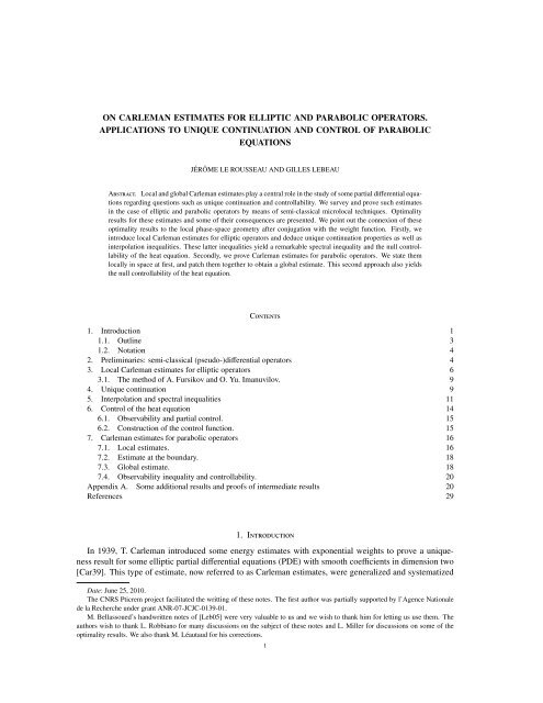
ON CARLEMAN ESTIMATES FOR ELLIPTIC AND PARABOLIC OPERATORS.<br />
APPLICATIONS TO UNIQUE CONTINUATION AND CONTROL OF PARABOLIC<br />
EQUATIONS<br />
JÉRÔME LE ROUSSEAU AND GILLES LEBEAU<br />
ABSTRACT. Local <strong>and</strong> global Carleman <strong>estimates</strong> play a central role in the study of some partial differential equati<strong>on</strong>s<br />
regarding questi<strong>on</strong>s such as unique c<strong>on</strong>tinuati<strong>on</strong> <strong>and</strong> c<strong>on</strong>trollability. We survey <strong>and</strong> prove such <strong>estimates</strong><br />
in the case of <strong>elliptic</strong> <strong>and</strong> <strong>parabolic</strong> <strong>operators</strong> by means of semi-classical microlocal techniques. Optimality<br />
results <strong>for</strong> these <strong>estimates</strong> <strong>and</strong> some of their c<strong>on</strong>sequences are presented. We point out the c<strong>on</strong>nexi<strong>on</strong> of these<br />
optimality results to the local phase-space geometry after c<strong>on</strong>jugati<strong>on</strong> with the weight functi<strong>on</strong>. Firstly, we<br />
introduce local Carleman <strong>estimates</strong> <strong>for</strong> <strong>elliptic</strong> <strong>operators</strong> <strong>and</strong> deduce unique c<strong>on</strong>tinuati<strong>on</strong> properties as well as<br />
interpolati<strong>on</strong> inequalities. These latter inequalities yield a remarkable spectral inequality <strong>and</strong> the null c<strong>on</strong>trollability<br />
of the heat equati<strong>on</strong>. Sec<strong>on</strong>dly, we prove Carleman <strong>estimates</strong> <strong>for</strong> <strong>parabolic</strong> <strong>operators</strong>. We state them<br />
locally in space at first, <strong>and</strong> patch them together to obtain a global estimate. This sec<strong>on</strong>d approach also yields<br />
the null c<strong>on</strong>trollability of the heat equati<strong>on</strong>.<br />
CONTENTS<br />
1. Introducti<strong>on</strong> 1<br />
1.1. Outline 3<br />
1.2. Notati<strong>on</strong> 4<br />
2. Preliminaries: semi-classical (pseudo-)differential <strong>operators</strong> 4<br />
3. Local Carleman <strong>estimates</strong> <strong>for</strong> <strong>elliptic</strong> <strong>operators</strong> 6<br />
3.1. The method of A. Fursikov <strong>and</strong> O. Yu. Imanuvilov. 9<br />
4. Unique c<strong>on</strong>tinuati<strong>on</strong> 9<br />
5. Interpolati<strong>on</strong> <strong>and</strong> spectral inequalities 11<br />
6. C<strong>on</strong>trol of the heat equati<strong>on</strong> 14<br />
6.1. Observability <strong>and</strong> partial c<strong>on</strong>trol. 15<br />
6.2. C<strong>on</strong>structi<strong>on</strong> of the c<strong>on</strong>trol functi<strong>on</strong>. 15<br />
7. Carleman <strong>estimates</strong> <strong>for</strong> <strong>parabolic</strong> <strong>operators</strong> 16<br />
7.1. Local <strong>estimates</strong>. 16<br />
7.2. Estimate at the boundary. 18<br />
7.3. Global estimate. 18<br />
7.4. Observability inequality <strong>and</strong> c<strong>on</strong>trollability. 20<br />
Appendix A. Some additi<strong>on</strong>al results <strong>and</strong> proofs of intermediate results 20<br />
References 29<br />
1. INTRODUCTION<br />
In 1939, T. Carleman introduced some energy <strong>estimates</strong> with exp<strong>on</strong>ential weights to prove a uniqueness<br />
result <strong>for</strong> some <strong>elliptic</strong> partial differential equati<strong>on</strong>s (PDE) with smooth coefficients in dimensi<strong>on</strong> two<br />
[Car39]. This type of estimate, now referred to as Carleman <strong>estimates</strong>, were generalized <strong>and</strong> systematized<br />
Date: June 25, 2010.<br />
The CNRS Pticrem project facilitated the writting of these notes. The first author was partially supported by l’Agence Nati<strong>on</strong>ale<br />
de la Recherche under grant ANR-07-JCJC-0139-01.<br />
M. Bellassoued’s h<strong>and</strong>written notes of [Leb05] were very valuable to us <strong>and</strong> we wish to thank him <strong>for</strong> letting us use them. The<br />
authors wish to thank L. Robbiano <strong>for</strong> many discussi<strong>on</strong>s <strong>on</strong> the subject of these notes <strong>and</strong> L. Miller <strong>for</strong> discussi<strong>on</strong>s <strong>on</strong> some of the<br />
optimality results. We also thank M. Léautaud <strong>for</strong> his correcti<strong>on</strong>s.<br />
1
2 JÉRÔME LE ROUSSEAU AND GILLES LEBEAU<br />
by L. Hörm<strong>and</strong>er <strong>and</strong> others <strong>for</strong> a large class of differential <strong>operators</strong> in arbitrary dimensi<strong>on</strong>s (see [Hör63,<br />
chapter 8] <strong>and</strong> [Hör85a, Secti<strong>on</strong>s 28.1-2]; see also [Zui83]).<br />
In more recent years, the field of applicati<strong>on</strong>s of Carleman <strong>estimates</strong> has g<strong>on</strong>e bey<strong>on</strong>d the original domain<br />
they had been introduced <strong>for</strong>, i.e., a quantitative result <strong>for</strong> unique c<strong>on</strong>tinuati<strong>on</strong>. They are also used in the<br />
study of inverse problems <strong>and</strong> c<strong>on</strong>trol theory <strong>for</strong> PDEs. Here, we shall mainly survey the applicati<strong>on</strong><br />
to c<strong>on</strong>trol theory in the case of <strong>parabolic</strong> equati<strong>on</strong>s, <strong>for</strong> which Carleman <strong>estimates</strong> have now become an<br />
essential technique.<br />
In c<strong>on</strong>trol of PDEs, <strong>for</strong> evoluti<strong>on</strong> equati<strong>on</strong>s, <strong>on</strong>e aims to drive the soluti<strong>on</strong> in a prescribed state, starting<br />
from a certain initial c<strong>on</strong>diti<strong>on</strong>. One acts <strong>on</strong> the equati<strong>on</strong> through a source term, a so-called distributed<br />
c<strong>on</strong>trol, or through a boundary c<strong>on</strong>diti<strong>on</strong>, a so-called boundary c<strong>on</strong>trol. To achieve general results <strong>on</strong>e<br />
wishes <strong>for</strong> the c<strong>on</strong>trol to <strong>on</strong>ly act in part of the domain or its boundary <strong>and</strong> <strong>on</strong>e wishes to have as much<br />
latitude as possible in the choice of the c<strong>on</strong>trol regi<strong>on</strong>: locati<strong>on</strong>, size.<br />
As already menti<strong>on</strong>ed, we focus our interest <strong>on</strong> the heat equati<strong>on</strong> here. In a smooth <strong>and</strong> bounded 1 domain<br />
Ω in R n , <strong>for</strong> a time interval (0, T) with T > 0, <strong>and</strong> <strong>for</strong> a distributed c<strong>on</strong>trol we c<strong>on</strong>sider<br />
⎧<br />
∂ t y − ∆y = 1 ω v in Q = (0, T) × Ω,<br />
⎪⎨<br />
(1.1)<br />
y = 0<br />
<strong>on</strong> Σ = (0, T) × ∂Ω,<br />
⎪⎩ y(0) = y 0 in Ω.<br />
Here ω ⋐ Ω is an interior c<strong>on</strong>trol regi<strong>on</strong>. The null c<strong>on</strong>trollability of this equati<strong>on</strong>, that is the existence, <strong>for</strong><br />
any y 0 ∈ L 2 (Ω), of a c<strong>on</strong>trol v ∈ L 2 (Q), with ‖v‖ L 2 (Q) ≤ C‖y 0 ‖ L 2 (Q), such that y(T) = 0, was first proven in<br />
[LR95], by means of Carleman <strong>estimates</strong> <strong>for</strong> the <strong>elliptic</strong> operator −∂ 2 s − ∆ x in a domain Z = (0, S 0 ) × Ω with<br />
S 0 > 0. A sec<strong>on</strong>d approach, introduced in [FI96], also led to the null c<strong>on</strong>trollability of the heat equati<strong>on</strong>.<br />
It is based <strong>on</strong> global Carleman <strong>estimates</strong> <strong>for</strong> the <strong>parabolic</strong> operator ∂ t − ∆. These <strong>estimates</strong> are said to be<br />
global <strong>for</strong> they apply to functi<strong>on</strong>s that are defined in the whole domain (0, T) × Ω <strong>and</strong> that solely satisfy<br />
boundary c<strong>on</strong>diti<strong>on</strong>, e.g., homogeneous Dirichlet boundary c<strong>on</strong>diti<strong>on</strong>s <strong>on</strong> (0, T) × ∂Ω.<br />
We shall first survey the approach of [LR95], proving <strong>and</strong> using local <strong>elliptic</strong> Carleman <strong>estimates</strong>. We<br />
prove such <strong>estimates</strong> with techniques from semi-classical microlocal analysis. The <strong>estimates</strong> we prove are<br />
local in the sense that they apply to functi<strong>on</strong>s whose support is localized in a closed regi<strong>on</strong> strictly included<br />
in Ω. With these <strong>estimates</strong> at h<strong>and</strong>, we derive interpolati<strong>on</strong> inequalities <strong>for</strong> functi<strong>on</strong>s in Z = (0, S 0 ) × Ω,<br />
that satisfy some boundary c<strong>on</strong>diti<strong>on</strong>s, <strong>and</strong> we derive a spectral inequality <strong>for</strong> finite linear combinati<strong>on</strong>s<br />
of eigenfuncti<strong>on</strong>s of the Laplace operator in Ω with homogeneous Dirichlet boundary c<strong>on</strong>diti<strong>on</strong>s. This<br />
yields an iterative c<strong>on</strong>structi<strong>on</strong> of the c<strong>on</strong>trol functi<strong>on</strong> v working in increasingly larger finite dimensi<strong>on</strong>al<br />
subspaces.<br />
The method introduced in [LR95] was further extended to address thermoelasticity [LZ98], thermoelastic<br />
plates [BN02], semigroups generated by fracti<strong>on</strong>al orders of <strong>elliptic</strong> <strong>operators</strong> [Mil06]. It has also been<br />
used to prove null c<strong>on</strong>trollability results in the case of n<strong>on</strong> smooth coefficients [BDL07b, LR09a]. Local<br />
Carleman <strong>estimates</strong> have also been central in the study of other types of PDEs <strong>for</strong> instance to prove unique<br />
c<strong>on</strong>tinuati<strong>on</strong> results [SS87, Rob91, FL96, Tat95b, Tat95a] <strong>and</strong> to prove stabilizati<strong>on</strong> results [LR97, Bel03]<br />
to cite a few. Here, we shall c<strong>on</strong>sider self-adjoint <strong>elliptic</strong> <strong>operators</strong>, in particular the Laplace operator. The<br />
method of [LR95] can also be extended to some n<strong>on</strong> selfadjoint case, e.g. n<strong>on</strong> symmetric systems [Léa09].<br />
In a sec<strong>on</strong>d part we survey the approach of [FI96], that is by means of global <strong>parabolic</strong> Carleman <strong>estimates</strong>.<br />
These <strong>estimates</strong> are characterized by an observati<strong>on</strong> term. Such an estimate readily yields a so-called<br />
observability inequality <strong>for</strong> the <strong>parabolic</strong> operator, which is equivalent to the null c<strong>on</strong>trollability of the linear<br />
system (1.1). The proof of <strong>parabolic</strong> Carleman <strong>estimates</strong> we provide is new <strong>and</strong> different from that given<br />
in [FI96]. In [FI96] the estimate is derived through numerous integrati<strong>on</strong>s by parts <strong>and</strong> the identificati<strong>on</strong> of<br />
positive “dominant” terms. As in the <strong>elliptic</strong> case of the first part, we base our analysis <strong>on</strong> semi-classical<br />
microlocal analysis. In particular, the estimate is obtained through a time-uni<strong>for</strong>m semi-classical Gårding<br />
inequality. In the case of <strong>parabolic</strong> <strong>operators</strong>, we first prove local <strong>estimates</strong> <strong>and</strong> we also show how such<br />
<strong>estimates</strong> can be patched together to finally yield a global estimate with an observati<strong>on</strong> term in the <strong>for</strong>m of<br />
that proved by [FI96].<br />
1 The problem of null-c<strong>on</strong>trollability of the heat equati<strong>on</strong> in the case where Ω is unbounded is entirely different [MZ01, Mil05, Mil].
CARLEMAN ESTIMATES 3<br />
The approach of [FI96] has been successful, allowing to also treat the c<strong>on</strong>trollability of more general<br />
<strong>parabolic</strong> equati<strong>on</strong>s. Time dependent terms can be introduced in the <strong>parabolic</strong> equati<strong>on</strong>. Moreover, <strong>on</strong>e<br />
may c<strong>on</strong>sider the c<strong>on</strong>trollability of some semi-linear <strong>parabolic</strong> equati<strong>on</strong>s. For these questi<strong>on</strong>s we refer to<br />
[FI96, Bar00, FCZ00b, DFCGBZ02]. In fact, global Carleman <strong>estimates</strong> yield a precise knowledge of the<br />
“cost” of the c<strong>on</strong>trol functi<strong>on</strong> in the linear case [FCZ00a] which allows to carry out a fix point argument after<br />
linearizati<strong>on</strong> of the semi-linear equati<strong>on</strong>. The results <strong>on</strong> semi-linear equati<strong>on</strong>s have been extended to the<br />
case of n<strong>on</strong> smooth coefficients [DOP02, BDL07a, Le 07, LR09b]. The use of global <strong>parabolic</strong> Carleman<br />
<strong>estimates</strong> has also allowed to address the c<strong>on</strong>trollability of n<strong>on</strong> linear equati<strong>on</strong>s such as the Navier-Stokes<br />
equati<strong>on</strong>s [Ima01, FCGIP04], the Boussinesq system [FCGIP06], fluid structure systems [IT07, BO08],<br />
weakly coupled <strong>parabolic</strong> systems [de 00, ABDK05, ABD06, GBPG06] to cite a few. A review of the<br />
applicati<strong>on</strong> of global <strong>parabolic</strong> Carleman <strong>estimates</strong> can be found in [FCG06].<br />
A local Carleman <strong>estimates</strong> takes the following <strong>for</strong>m. For an <strong>elliptic</strong> operator P <strong>and</strong> <strong>for</strong> a well-chosen<br />
weight functi<strong>on</strong> ϕ = ϕ(x), there exists C > 0 <strong>and</strong> h 1 > 0 such that<br />
(1.2)<br />
h‖e ϕ/h u‖ 2 0 + h 3 ‖e ϕ/h ∇ x u‖ 2 0 ≤ Ch 4 ‖e ϕ/h Pu‖ 2 0,<br />
<strong>for</strong> u smooth with compact support <strong>and</strong> 0 < h ≤ h 1 .<br />
In this type of estimate we can take the parameter h as small as needed, which is often d<strong>on</strong>e in applicati<strong>on</strong>s<br />
to inverse problems or c<strong>on</strong>trol theory. For this reas<strong>on</strong>, it appeared sensible to us to present results<br />
regarding the optimality of the powers of the parameter h in such Carleman <strong>estimates</strong>. For example, in the<br />
case of <strong>parabolic</strong> <strong>estimates</strong> this questi<strong>on</strong> is crucial <strong>for</strong> the applicati<strong>on</strong> to the c<strong>on</strong>trollability of semilinear<br />
<strong>parabolic</strong> equati<strong>on</strong>s (see e.g. [FCZ00b, DFCGBZ02]). To make precise such optimality result we present<br />
its c<strong>on</strong>necti<strong>on</strong> to the local phase-space geometry. We show that the presences of h in fr<strong>on</strong>t of the first term<br />
<strong>and</strong> h 3 in fr<strong>on</strong>t of the sec<strong>on</strong>d term in (1.2) are c<strong>on</strong>nected to the characteristic set of the c<strong>on</strong>jugated operator<br />
P ϕ = h 2 e ϕ/h Pe −ϕ/h . Away from this characteristic set, a better estimate can be achieved.<br />
If ω is an open subset of Ω, from <strong>elliptic</strong> Carleman <strong>estimates</strong> we obtain a spectral inequality of the <strong>for</strong>m<br />
‖u‖ 2 L 2 (Ω) ≤ CeC √µ ‖u‖ 2 L 2 (ω) ,<br />
<strong>for</strong> some C > 0 <strong>and</strong> <strong>for</strong> u a linear combinati<strong>on</strong> of eigenfuncti<strong>on</strong>s of −∆ associated to eigenvalues less than<br />
µ > 0. An optimality result <strong>for</strong> such an inequality is also presented as well as some unique c<strong>on</strong>tinuati<strong>on</strong><br />
property <strong>for</strong> series of eigenfuncti<strong>on</strong>s of −∆. This spectral inequality is also at the center of the c<strong>on</strong>structi<strong>on</strong><br />
of the c<strong>on</strong>trol functi<strong>on</strong> of (1.1) <strong>and</strong> the estimati<strong>on</strong> of its “cost” <strong>for</strong> particular frequency ranges.<br />
An important point in the derivati<strong>on</strong> of a Carleman estimate c<strong>on</strong>sist in the choice of the weight functi<strong>on</strong><br />
ϕ. A necessary c<strong>on</strong>diti<strong>on</strong> can be derived. This c<strong>on</strong>diti<strong>on</strong> c<strong>on</strong>cerns the sub-<strong>elliptic</strong>ity of the symbol of the<br />
c<strong>on</strong>jugated operator P ϕ . With the approach we use, the sufficiency of this c<strong>on</strong>diti<strong>on</strong> is obtained 2 . We also<br />
c<strong>on</strong>sider str<strong>on</strong>ger sufficient c<strong>on</strong>diti<strong>on</strong>s. The method introduced by [FI96] to derive Carleman <strong>estimates</strong> is<br />
analyzed in this framework.<br />
Here, we shall <strong>on</strong>ly prove estimate in the interior, away from the boundary of Ω. For proofs of Carleman<br />
<strong>estimates</strong> at the boundary we shall refer the reader to the original articles.<br />
This article originates in part from a lecture given by G. Lebeau at the Faculté des Sciences in Tunis in<br />
February 2005 <strong>and</strong> from M. Bellassoued’s h<strong>and</strong>written notes taken <strong>on</strong> this occasi<strong>on</strong> [Leb05].<br />
1.1. Outline. We start by briefly introducing semi-classical pseudodifferential <strong>operators</strong> (ψDO) in Secti<strong>on</strong><br />
2. The Gårding inequality will be <strong>on</strong>e of the important tools we introduce. It will allow us to quickly<br />
derive a local Carleman estimate <strong>for</strong> an <strong>elliptic</strong> operator in Secti<strong>on</strong> 3. In that secti<strong>on</strong>, we present the sub<strong>elliptic</strong>ity<br />
c<strong>on</strong>diti<strong>on</strong> that the weight functi<strong>on</strong> has to fulfill. We also show the optimality of the powers of the<br />
semi-classical parameter h in the Carleman <strong>estimates</strong>. We apply Carleman <strong>estimates</strong> to <strong>elliptic</strong> equati<strong>on</strong>s<br />
<strong>and</strong> inequalities <strong>and</strong> prove unique c<strong>on</strong>tinuati<strong>on</strong> results in Secti<strong>on</strong> 4. In Secti<strong>on</strong> 5, we prove the interpolati<strong>on</strong><br />
<strong>and</strong> spectral inequalities. The latter inequality c<strong>on</strong>cerns finite linear combinati<strong>on</strong>s of eigenfuncti<strong>on</strong>s of<br />
the <strong>elliptic</strong> operator. We show the optimality of the c<strong>on</strong>stant e C √µ in this inequality where µ is the largest<br />
eigenvalue c<strong>on</strong>sidered in the sum. We also prove a unique c<strong>on</strong>tinuati<strong>on</strong> property <strong>for</strong> some series of such<br />
2 This is proven in the <strong>elliptic</strong> case here. In the <strong>parabolic</strong> case a more involved analysis is needed. It can be found in [LR09b].
4 JÉRÔME LE ROUSSEAU AND GILLES LEBEAU<br />
eigenfuncti<strong>on</strong>s. In Secti<strong>on</strong> 6, these results are applied to c<strong>on</strong>struct a c<strong>on</strong>trol functi<strong>on</strong> <strong>for</strong> the <strong>parabolic</strong> equati<strong>on</strong><br />
(1.1). Secti<strong>on</strong> 7 is devoted to <strong>parabolic</strong> Carleman <strong>estimates</strong>. We first prove them locally in space with<br />
a uni<strong>for</strong>m-in-time Gårding inequality. We then patch them together to obtain a global estimate. We provide<br />
a sec<strong>on</strong>d proof of the null c<strong>on</strong>trollability of <strong>parabolic</strong> equati<strong>on</strong>s with this approach.<br />
For a clearer expositi<strong>on</strong>, some of the results given in the main secti<strong>on</strong>s are proven in the appendices.<br />
1.2. Notati<strong>on</strong>. The notati<strong>on</strong> we use is classical. The can<strong>on</strong>ical inner product <strong>on</strong> R n is denoted by 〈., .〉,<br />
the associated Euclidean norm by |.| <strong>and</strong> the Euclidean open ball with center x <strong>and</strong> radius r by B(x, r). For<br />
ξ ∈ R n we set 〈ξ〉 := (1 + |ξ| 2 ) 1 2 . If α is a multi-index, i.e., α = (α 1 , . . . , α n ) ∈ N n , we introduce<br />
ξ α = ξ α 1<br />
1 · · · ξα n<br />
n , if ξ ∈ R n , ∂ α = ∂ α 1<br />
x 1 · · · ∂ α n<br />
x n<br />
, D α = D α 1<br />
x 1 · · · D α n<br />
x n<br />
, <strong>and</strong> |α| = α 1 + · · · + α n ,<br />
where D = h i ∂. In Rn , we denote by ∇ the gradient (∂ x1 , . . . , ∂ xn ) t <strong>and</strong> by ∆ the Laplace operator ∂ 2 x 1<br />
+· · ·+∂ 2 x n<br />
.<br />
If needed the variables al<strong>on</strong>g which differentiati<strong>on</strong>s are per<strong>for</strong>med will be made clear by writing ∇ x or ∆ x<br />
<strong>for</strong> instance. We shall also write ϕ ′ = ∇ x ϕ.<br />
For an open set Ω in R n , we denote by Cc ∞ (Ω) the set of functi<strong>on</strong>s of class C ∞ whose support is a compact<br />
subset of Ω. For a compact set K in R n , we denote by Cc ∞ (K) the set of functi<strong>on</strong>s in Cc ∞ (R n ) whose support<br />
is in K. The Schwartz space S (R n ) is the set of functi<strong>on</strong>s of class C ∞ that decrease rapidly at infinity. Its<br />
dual, S ′ (R n ), is the set of tempered distributi<strong>on</strong>s. The Fourier trans<strong>for</strong>m of a functi<strong>on</strong> u ∈ S (R n ) is defined<br />
by û(ξ) = ∫ e −i〈x,ξ〉 u(x) dx, with an extensi<strong>on</strong> by duality to S ′ (R n ).<br />
Let Ω be an open subset of R n . The space L 2 (Ω) of square integrable functi<strong>on</strong>s is equipped with the<br />
hermitian inner product (u, v) L 2 = ∫ Ω u(x)v(x) dx <strong>and</strong> the associated norm ‖u‖ L 2 = ‖u‖ 0 = (u, u) 1/2<br />
L 2 . In R n ,<br />
classical Sobolev spaces are defined by H s (R n ) = {u ∈ S ′ (R n ); 〈ξ〉 s û ∈ L 2 (R n )} <strong>for</strong> all s ∈ R. In Ω, <strong>for</strong><br />
s ∈ N, H s (Ω) is defined by H s (Ω) = {u ∈ D ′ (Ω); ∂ α u ∈ L 2 (R n ), ∀α ∈ N n , |α| ≤ s}.<br />
For two functi<strong>on</strong>s f <strong>and</strong> g with variables x, ξ in R n × R n , we defined their so-called Poiss<strong>on</strong> bracket<br />
{ f, g} = ∑ (∂ ξ j<br />
f ∂ x j<br />
g − ∂ x j<br />
f ∂ ξ j<br />
g).<br />
j<br />
For two <strong>operators</strong> A, B their commutator will be denoted [A, B] = AB − BA.<br />
In these notes, C will always denote a generic positive c<strong>on</strong>stant whose value can be different in each line.<br />
If we want to keep track of the value of a c<strong>on</strong>stant we shall use other letters. We shall sometimes write C λ<br />
<strong>for</strong> a generic c<strong>on</strong>stant that depends <strong>on</strong> a parameter λ.<br />
2. PRELIMINARIES: SEMI-CLASSICAL (PSEUDO-)DIFFERENTIAL OPERATORS<br />
Semi-classical theory originates from quantum physics. The scaling parameter h we introduce is c<strong>on</strong>sistent<br />
with Plank’s c<strong>on</strong>stant in physics. It will be assumed small: h ∈ (0, h 0 ), 0 < h 0
CARLEMAN ESTIMATES 5<br />
Lemma 2.2. Let m ∈ R <strong>and</strong> a j ∈ S m− j with j ∈ N. Then there exists a ∈ S m such that<br />
∀N ∈ N,<br />
∑<br />
a − N h j a j ∈ h N+1 S m−N−1 .<br />
j=0<br />
We then write a ∼ ∑ j h j a j . The symbol a is unique up to O(h ∞ )S −∞ , in the sense that the difference of two<br />
such symbols is in O(h N )S −M <strong>for</strong> all N, M ∈ N.<br />
We identify a 0 with the principal symbol of a. In general, <strong>for</strong> the symbols of the <strong>for</strong>m a ∼ ∑ j h j a j that<br />
we shall c<strong>on</strong>sider here the symbols a j will not depend <strong>on</strong> the scaling parameter h.<br />
With these symbol classes we can define pseudodifferential <strong>operators</strong> (ψDOs).<br />
Definiti<strong>on</strong> 2.3. If a ∈ S m , we set<br />
a(x, D, h)u(x) = Op(a)u(x) := (2πh) −n ∫∫ e i〈x−y,ξ〉/h a(x, ξ, h) u(y) dy dξ<br />
= (2πh) −n ∫ e i〈x,ξ〉/h a(x, ξ, h) û(ξ/h) dξ.<br />
We denote by Ψ m the set of these ψDOs. For A ∈ Ψ m , σ(A) will be its principal symbol.<br />
We have Op(a) : S (R n ) → S (R n ) c<strong>on</strong>tinuously <strong>and</strong> Op(a) can be uniquely extended to S ′ (R n ). Then<br />
Op(a) : S ′ (R n ) → S ′ (R n ) c<strong>on</strong>tinuously.<br />
Example 2.4. C<strong>on</strong>sider the differential operator defined by A = −h 2 ∆+V(x)+h 2 ∑ 1≤ j≤n b j (x)∂ j . Its symbol<br />
<strong>and</strong> principal symbol are a(x, ξ, h) = |ξ| 2 + V(x) + ih ∑ 1≤ j≤n b j (x)ξ j <strong>and</strong> σ(A) = |ξ| 2 + V(x) respectively.<br />
We now introduce Sobolev spaces <strong>and</strong> Sobolev norms which are adapted to the scaling parameter h. The<br />
natural norm <strong>on</strong> L 2 (R n ) is written as ‖u‖ 2 0 := ( ∫ |u(x)| 2 dx) 1 2 . Let s ∈ R; we then set<br />
‖u‖ s := ‖Λ s u‖ 0 , with Λ s := Op(〈ξ〉 s ) <strong>and</strong> H s (R n ) := {u ∈ S ′ (R n ); ‖u‖ s < ∞}.<br />
The space H s (R n ) is algebraically equal to the classical Sobolev space H s (R n ). For a fixed value of h, the<br />
norm ‖.‖ s is equivalent to the classical Sobolev norm that we write ‖.‖ H s. However, these norms are not<br />
uni<strong>for</strong>mly equivalent as h goes to 0. In fact we <strong>on</strong>ly have<br />
‖u‖ s ≤ C‖u‖ H s, if s ≥ 0, <strong>and</strong> ‖u‖ H s ≤ C‖u‖ s , if s ≤ 0.<br />
For s ∈ N the norm ‖.‖ s is equivalent to the norm N s (u) := ∑ |α|≤s ‖D α u‖ 2 0 = ∑ |α|≤s h 2|α| ‖∂ α u‖ 2 0 . The spaces<br />
H s <strong>and</strong> H −s are in duality, i.e. H −s = (H s ) ′ in the sense of distributi<strong>on</strong>al duality with L 2 = H 0 as a<br />
pivot space. We can prove the following c<strong>on</strong>tinuity result.<br />
Theorem 2.5. If a(x, ξ, h) ∈ S m <strong>and</strong> s ∈ R, we then have Op(a) : H s → H s−m c<strong>on</strong>tinuously, uni<strong>for</strong>mly in<br />
h.<br />
The following Gårding inequality is the important result we shall be interested in here.<br />
Theorem 2.6 (Gårding inequality). Let K be a compact set of R n . If a(x, ξ, h) ∈ S m , with principal part a m ,<br />
if there exists C > 0 such that<br />
Re a m (x, ξ, h) ≥ C〈ξ〉 m , x ∈ K, ξ ∈ R n , h ∈ (0, h 0 ),<br />
then <strong>for</strong> 0 < C ′ < C <strong>and</strong> h 1 > 0 sufficiently small we have<br />
Re(Op(a)u, u) ≥ C ′ ‖u‖ 2 m/2 ,<br />
u ∈ C ∞<br />
c (K), 0 < h ≤ h 1 .<br />
The positivity of the principal symbol of a thus implies a certain positivity <strong>for</strong> the operator Op(a). The<br />
value of h 1 depends <strong>on</strong> C, C ′ <strong>and</strong> a finite number of c<strong>on</strong>stants C α,β associated to the symbol a(x, ξ, h) (see<br />
Definiti<strong>on</strong> 2.1). A proof of the Gårding inequality is provided in Appendix A.<br />
Remark 2.7. We note here that the positivity c<strong>on</strong>diti<strong>on</strong> <strong>on</strong> the principal symbol is imposed <strong>for</strong> all ξ in R n ,<br />
as opposed to the assumpti<strong>on</strong>s made <strong>for</strong> the usual Gårding inequality, i.e., n<strong>on</strong> semi-classical, that <strong>on</strong>ly ask<br />
<strong>for</strong> such a positivity <strong>for</strong> |ξ| large (see e.g. [Tay81, Chapter 2]). The semi-classical result is however str<strong>on</strong>ger<br />
in the sense that it yields a true positivity <strong>for</strong> the operator.
6 JÉRÔME LE ROUSSEAU AND GILLES LEBEAU<br />
We shall compose ψDOs in the sequel. Such compositi<strong>on</strong>s yield a calculus at the level of operator<br />
symbols.<br />
Theorem 2.8 (Symbol calculus). Let a ∈ S m <strong>and</strong> b ∈ S m′ . Then Op(a) ◦ Op(b) = Op(c) <strong>for</strong> a certain<br />
c ∈ S m+m′ that admits the following asymptotic expansi<strong>on</strong><br />
c(x, ξ, h) = (a ♯ b)(x, ξ, h) ∼ ∑ α<br />
h |α|<br />
i |α| α! ∂α ξ a(x, ξ, h) ∂α xb(x, ξ, h), where α! = α 1 ! · · · α n !<br />
The first term in the expansi<strong>on</strong>, the principal symbol, is ab; the sec<strong>on</strong>d term is h i<br />
It follows that the principal symbol of the commutator [Op(a), Op(b)] is<br />
σ([Op(a), Op(b)]) = h i {a, b} ∈ hS m+m′ −1 .<br />
Finally, the symbol of the adjoint operator can be obtained as follows.<br />
∑<br />
j ∂ ξ j<br />
a(x, ξ, h) ∂ x j<br />
b(x, ξ, h).<br />
Theorem 2.9. Let a ∈ S m . Then Op(a) ∗ = Op(b) <strong>for</strong> a certain b ∈ S m that admits the following asymptotic<br />
expansi<strong>on</strong><br />
b(x, ξ, h) ∼ ∑ h |α|<br />
α i |α| α! ∂α ξ ∂α xa(x, ξ, h).<br />
The principal symbol of b is simply a.<br />
For references <strong>on</strong> usual ψDOs the reader can c<strong>on</strong>sult [Tay81, Hör85b, AG91, GS94, Shu01]. For references<br />
<strong>on</strong> semi-classical ψDOs the reader can c<strong>on</strong>sult [Rob87, DS99, Mar02].<br />
3. LOCAL CARLEMAN ESTIMATES FOR ELLIPTIC OPERATORS<br />
We shall prove a local Carleman <strong>estimates</strong> <strong>for</strong> a sec<strong>on</strong>d-order <strong>elliptic</strong> operator. To simplify notati<strong>on</strong> we<br />
c<strong>on</strong>sider the Laplace operator P = −∆ but the method we expose extends to more general sec<strong>on</strong>d-order<br />
<strong>elliptic</strong> <strong>operators</strong> with a principal part of the <strong>for</strong>m ∑ i, j ∂ j (a i j (x)∂ i ) with a i j ∈ C ∞ (R n , R), 1 ≤ i, j ≤ n <strong>and</strong><br />
∑<br />
i, j a i j (x)ξ i ξ j ≥ C|ξ| 2 , with C > 0, <strong>for</strong> all x, ξ ∈ R n . In particular, we note that Carleman <strong>estimates</strong> are<br />
insensitive 3 to changes in the operator by zero- or first-order terms.<br />
Let ϕ(x) be a real-valued functi<strong>on</strong>. We define the following c<strong>on</strong>jugated operator P ϕ = h 2 e ϕ/h Pe −ϕ/h to be<br />
c<strong>on</strong>sidered as a semi-classical differential operator. We have P ϕ = −h 2 ∆ − |ϕ ′ | 2 + 2〈ϕ ′ , h∇〉 + h∆ϕ. Its full<br />
symbol is given by |ξ| 2 − |ϕ ′ | 2 + 2i〈ϕ ′ , ξ〉 + h∆ϕ. Its principal symbol is given by<br />
p ϕ = σ(P ϕ ) = |ξ| 2 − |ϕ ′ | 2 + 2i〈ϕ ′ , ξ〉 = ∑ (ξ j + iϕ ′ x j<br />
) 2 ,<br />
j<br />
i.e., we have “replaced” ξ j by ξ j + iϕ ′ x j<br />
. In fact we note that the symbol of e ϕ/h D j e −ϕ/h is ξ j + iϕ ′ x j<br />
.<br />
We define the following symmetric <strong>operators</strong> Q 2 = (P ϕ + P ∗ ϕ)/2, Q 1 = (P ϕ − P ∗ ϕ)/(2i), with respective<br />
principal symbols<br />
q 2 = |ξ| 2 − |ϕ ′ | 2 , q 1 = 2〈ξ, ϕ ′ 〉.<br />
We have p ϕ = q 2 + iq 1 <strong>and</strong> P ϕ = Q 2 + iQ 1 .<br />
We choose ϕ that satisfies the following assumpti<strong>on</strong>.<br />
Assumpti<strong>on</strong> 3.1 (L. Hörm<strong>and</strong>er [Hör63, Hör85a]). Let V be a bounded open set in R n . We say that the<br />
weight functi<strong>on</strong> ϕ ∈ C ∞ (R n , R) satisfies the sub-<strong>elliptic</strong>ity assumpti<strong>on</strong> in V if |ϕ ′ | > 0 in V <strong>and</strong><br />
∀(x, ξ) ∈ V × R n , p ϕ (x, ξ) = 0 ⇒ {q 2 , q 1 }(x, ξ) ≥ C > 0.<br />
Remark 3.2. We note that p ϕ (x, ξ) = 0 is equivalent to |ξ| = |ϕ ′ | <strong>and</strong> 〈ξ, ϕ ′ 〉 = 0. In particular, the<br />
characteristic set Z = {(x, ξ) ∈ V × R n ; p ϕ (x, ξ) = 0} is compact as illustrated in Figure 1.<br />
Assumpti<strong>on</strong> 3.1 can be fulfilled as stated in the following lemma whose proof can be found in Appendix<br />
A.<br />
3 In the sense that <strong>on</strong>ly c<strong>on</strong>stants are affected. In Theorem 3.5 below the c<strong>on</strong>stants C <strong>and</strong> h1 change but not the <strong>for</strong>m of the estimate.
CARLEMAN ESTIMATES 7<br />
ϕ ′ (x)<br />
0<br />
p ϕ = 0<br />
Figure 1: Form of the characteristic set Z at the vertical of each point x ∈ V.<br />
Lemma 3.3 (L. Hörm<strong>and</strong>er [Hör63, Hör85a]). Let V be a bounded open set in R n <strong>and</strong> ψ ∈ C ∞ (R n , R) be<br />
such that |ψ ′ | > 0 in V. Then ϕ = e λψ fulfills Assumpti<strong>on</strong> 3.1 in V <strong>for</strong> λ > 0 sufficiently large.<br />
The proof of the Carleman estimate will make use of the Gårding inequality. In preparati<strong>on</strong>, we have the<br />
following result proven in Appendix A that follows from Assumpti<strong>on</strong> 3.1.<br />
Lemma 3.4. Let µ > 0 <strong>and</strong> ρ = µ(q 2 2 + q2 1 ) + {q 2, q 1 }. Then, <strong>for</strong> all (x, ξ) ∈ V × R n , we have ρ(x, ξ) ≥ C〈ξ〉 4 ,<br />
with C > 0, <strong>for</strong> µ sufficiently large.<br />
We may now prove the following Carleman estimate.<br />
Theorem 3.5. Let V be a bounded open set in R n <strong>and</strong> let ϕ satisfy Assumpti<strong>on</strong> 3.1 in V; then, there exist<br />
0 < h 1 < h 0 <strong>and</strong> C > 0 such that<br />
(3.1)<br />
h‖e ϕ/h u‖ 2 0 + h 3 ‖e ϕ/h ∇ x u‖ 2 0 ≤ Ch 4 ‖e ϕ/h Pu‖ 2 0,<br />
<strong>for</strong> u ∈ C ∞<br />
c (V) <strong>and</strong> 0 < h < h 1 .<br />
Proof. We set v = e ϕ/h u. Then, Pu = f is equivalent to P ϕ v = g = h 2 e ϕ/h f or rather Q 2 v + iQ 1 v = g.<br />
Observing that (Q j w 1 , w 2 ) = (w 1 , Q j w 2 ) <strong>for</strong> w 1 , w 2 ∈ Cc ∞ (R n ) we then obtain<br />
((<br />
(3.2) ‖g‖ 2 0 = ‖Q 1v‖ 2 0 + ‖Q 2v‖ 2 0 + 2 Re(Q 2v, iQ 1 v) = Q<br />
2<br />
1 + Q 2 2 + i[Q 2, Q 1 ] ) v, v)<br />
.<br />
We choose µ > 0 as given in Lemma 3.4. Then, <strong>for</strong> h such that hµ ≤ 1 we have<br />
((<br />
h µ(Q<br />
2<br />
1 + Q 2 2 ) + i h [Q 2, Q 1 ] ) )<br />
v, v ≤ ‖g‖ 2 0 .<br />
}{{}<br />
principal symbol = µ(q 2 1 +q2 2 )+{q 2,q 1 }<br />
The Gårding inequality <strong>and</strong> Lemma 3.4 then yield<br />
(3.3) h‖v‖ 2 2 ≤ C‖g‖2 0 .<br />
We c<strong>on</strong>tent 4 ourselves with the norm in H 1 here <strong>and</strong> we obtain h‖e ϕ/h u‖ 2 0 + h 3 ‖∇ x (e ϕ/h u)‖ 2 0 ≤ Ch 4 ‖e ϕ/h f ‖ 2 0.<br />
We write ∇ x (e ϕ/h u) = h −1 e ϕ/h (∇ x ϕ)u + e ϕ/h ∇ x u, which yields<br />
since |∇ x ϕ| ≤ C. This c<strong>on</strong>cludes the proof.<br />
h 3 ‖e ϕ/h ∇ x u‖ 2 0 ≤ Ch‖e ϕ/h u‖ 2 0 + Ch 3 ‖∇ x (e ϕ/h u)‖ 2 0,<br />
<br />
4 Note that in the <strong>elliptic</strong> regi<strong>on</strong>, e.g. <strong>for</strong> large |ξ|, we can obtain a better result without the factor h in (3.3). In the neighborhood<br />
of the characteristic set Z = {p ϕ = 0} the choice of the norm in H 1 or H 2 matters very little since this regi<strong>on</strong> is compact. See<br />
Propositi<strong>on</strong> 3.8 <strong>for</strong> more details.
8 JÉRÔME LE ROUSSEAU AND GILLES LEBEAU<br />
supp( χ 1 )<br />
supp( χ 2 )<br />
Z<br />
V × R n<br />
Figure 2: Characteristic set Z <strong>and</strong> supports of χ 1 <strong>and</strong> χ 2 in Propositi<strong>on</strong> 3.8.<br />
Remark 3.6. With a density argument the result of Theorem 3.5 can be extended to functi<strong>on</strong>s u ∈ H 2 0 (V).<br />
However, here, we do not treat the case of functi<strong>on</strong>s in H 1 0 (V) ∩ H2 (V). For such a result <strong>on</strong>e needs a<br />
local Carleman estimate at the boundary of the open set V as proven in [LR95, Propositi<strong>on</strong> 2 page 351].<br />
Moreover, a global estimate in V <strong>for</strong> a functi<strong>on</strong> u in H 1 0 (V) ∩ H2 (V) requires an observati<strong>on</strong> term in the<br />
r.h.s. of the Carleman estimate. We shall provide such details in the case of <strong>parabolic</strong> <strong>operators</strong> below (see<br />
Secti<strong>on</strong> 7).<br />
Remark 3.7. In the proof of Theorem 3.5 we have used Assumpti<strong>on</strong> 3.1. We give complementary roles to<br />
the square terms in (3.2), ‖Q 1 u‖ 2 0 <strong>and</strong> ‖Q 2u‖ 2 0 , <strong>and</strong> to the acti<strong>on</strong> of the commutator i([Q 2, Q 1 ]u, u). As the<br />
square terms approach zero, the commutator term comes into effect <strong>and</strong> yields positivity. A. Fursikov <strong>and</strong><br />
O. Yu. Imanuvilov [FI96] have introduced a modificati<strong>on</strong> of the proof that allows to <strong>on</strong>ly c<strong>on</strong>sider a term<br />
equivalent to the commutator term without using the two square terms. This approach is presented below.<br />
The following propositi<strong>on</strong> yields a more precise result than the previous Carleman estimate <strong>and</strong> illustrates<br />
the loss of a half derivative in the neighborhood of the characteristic set Z .<br />
Propositi<strong>on</strong> 3.8. Let s ∈ R <strong>and</strong> V be a bounded open set in R n <strong>and</strong> let ϕ satisfy Assumpti<strong>on</strong> 3.1 in V. Let<br />
χ 1 , χ 2 ∈ S 0 with compact supports in x. Assume that χ 1 vanishes in a neighborhood of Z <strong>and</strong> that χ 2<br />
vanishes outside a compact neighborhood of Z . Then there exist C > 0 <strong>and</strong> 0 < h 2 < h 0 such that<br />
(3.4)<br />
‖Op( χ 1 )v‖ 2 ≤ C ( ‖P ϕ v‖ 0<br />
+ h‖v‖ 1<br />
)<br />
, <strong>and</strong> h<br />
1<br />
2 ‖Op( χ2 )v‖ s ≤ C ( ‖P ϕ v‖ 0<br />
+ h‖v‖ 1<br />
)<br />
,<br />
<strong>for</strong> v ∈ C ∞<br />
c (V) <strong>and</strong> 0 < h < h 2 .<br />
This propositi<strong>on</strong> is proven in Appendix A.5. We take χ 1 <strong>and</strong> χ 2 that satisfy the assumpti<strong>on</strong>s made<br />
in Propositi<strong>on</strong> 3.8 <strong>and</strong> such that χ 1 + χ 2 = 1 in a neighborhood of V × R n . For v ∈ Cc ∞ (V) we have<br />
‖Op(1 − χ 1 − χ 2 )v‖ r ≤ C N,r,r ′h N ‖v‖ r ′ <strong>for</strong> all N ∈ N <strong>and</strong> r, r ′ ∈ R. We thus obtain<br />
h 1 2 ‖v‖2 ≤ h 1 2 (‖Op(1 − χ1 − χ 2 )v‖ 2 + ‖Op( χ 1 )v‖ 2 + ‖Op( χ 2 )v‖ 2 ) ≤ C ( ‖P ϕ v‖ 0<br />
+ h‖v‖ 1<br />
)<br />
.<br />
Choosing h sufficiently small we obtain<br />
(3.5)<br />
h 1 2 ‖v‖2 ≤ C ′ ‖P ϕ v‖ 0<br />
,<br />
which brings us back to the last step in the proof of Theorem 3.5. Also note that (3.5) allows us to remove<br />
the sec<strong>on</strong>d term in the r.h.s. in each inequalities in (3.4) <strong>and</strong> we thus obtain<br />
(3.6)<br />
‖Op( χ 1 )v‖ 2 ≤ C‖P ϕ v‖ 0<br />
, <strong>and</strong> h 1 2 ‖Op( χ2 )v‖ s ≤ C‖P ϕ v‖ 0<br />
.<br />
We have seen that the sub-<strong>elliptic</strong>ity c<strong>on</strong>diti<strong>on</strong> in Assumpti<strong>on</strong> 3.1 is sufficient to obtain a Carleman<br />
estimate in Theorem 3.5. In fact we can prove that this c<strong>on</strong>diti<strong>on</strong> is necessary. We also note that the powers<br />
of the factors h in the l.h.s. of the estimate in Theorem 3.5 as well as in the sec<strong>on</strong>d inequality in (3.6) are<br />
optimal: <strong>for</strong> instance, we may not have h 2α in fr<strong>on</strong>t of the first term in inequality (3.1) with α < 1 2 . These<br />
two points are summarized in the following propositi<strong>on</strong>.
CARLEMAN ESTIMATES 9<br />
Propositi<strong>on</strong> 3.9. Let V be a bounded open set in R n , ϕ(x) ∈ C ∞ (R n , R), 0 < h 1 < h 0 <strong>and</strong> C > 0 such that<br />
<strong>for</strong> a certain α ≤ 1 2 we have<br />
(3.7)<br />
h α ‖e ϕ/h u‖ 0 ≤ Ch 2 ‖e ϕ/h Pu‖ 0 ,<br />
<strong>for</strong> all u ∈ Cc ∞ (V) <strong>and</strong> 0 < h < h 1 . Then α = 1 2<br />
<strong>and</strong> the weight functi<strong>on</strong> ϕ satisfies Assumpti<strong>on</strong> 3.1 in V.<br />
The reader is referred to Appendix A.6 <strong>for</strong> a proof.<br />
3.1. The method of A. Fursikov <strong>and</strong> O. Yu. Imanuvilov. Following the approach introduced by A. Fursikov<br />
<strong>and</strong> O. Yu. Imanuvilov [FI96], we provide an alternative proof of Theorem 3.5 in the <strong>elliptic</strong> case. We<br />
use the notati<strong>on</strong> of the proof of Theorem 3.5, <strong>and</strong> write<br />
‖g + µh∆ϕv‖ 2 0 = ‖Q 2v‖ 2 0 + ‖ ˜Q 1 v‖ 2 0 + (i[Q 2 , Q 1 ]v, v) + 2 Re(Q 2 v, µh∆ϕv), 0 < µ ≤ 2.<br />
where ˜Q 1 = Q 1 − iµh∆ϕ <strong>and</strong> we obtain ‖g + µh∆ϕv‖ 2 0 = ‖Q 2v‖ 2 0 + ‖ ˜Q 1 v‖ 2 0 + h Re(Rv, v), where ρ = σ(R) =<br />
({q 2 , q 1 } + 2µq 2 ∆ϕ). We have the following lemma, which proof can be found in Secti<strong>on</strong> A.4.<br />
Lemma 3.10. If ϕ = e λψ , then <strong>for</strong> λ > 0 sufficiently large, there exists C λ > 0 such that<br />
ρ = {q 2 , q 1 } + 2µq 2 ∆ϕ ≥ C λ 〈ξ〉 2 , x ∈ V, ξ ∈ R n .<br />
With the Gårding inequality we then c<strong>on</strong>clude that Re(Rv, v) ≥ C ′ ‖v‖ 2 1 , <strong>for</strong> 0 < C′ < C λ <strong>and</strong> h taken<br />
sufficiently small. The Carleman estimate follows without using the square terms ‖Q 2 v‖ 2 0 <strong>and</strong> ‖ ˜Q 1 v‖ 2 0. In<br />
fact we write<br />
‖g + µh∆ϕv‖ 2 0 ≤ 2‖g‖2 0 + 2µ2 h 2 ‖∆ϕv‖ 2 0 ,<br />
<strong>and</strong> the sec<strong>on</strong>d term in the r.h.s. can be “absorbed” by h‖v‖ 2 1 <strong>for</strong> h sufficiently small.<br />
<br />
Remark 3.11. The method of A. Fursikov <strong>and</strong> O. Yu. Imanuvilov, at the symbol level, is a matter of adding<br />
a term of the <strong>for</strong>m 2µq 2 ∆ϕ to the commutator symbol i h [Q 2, Q 1 ]. As the sign of q 2 ∆ϕ is not fixed, a precise<br />
choice of the value of µ is crucial.<br />
In the proof of Lemma 3.3 in Secti<strong>on</strong> A.2 we in fact obtained the following c<strong>on</strong>diti<strong>on</strong> <strong>on</strong> the weight<br />
functi<strong>on</strong><br />
(3.8) ∀(x, ξ) ∈ V × R n , q 2 (x, ξ) = 0 ⇒ {q 2 , q 1 }(x, ξ) ≥ C > 0.<br />
which is str<strong>on</strong>ger that the c<strong>on</strong>diti<strong>on</strong> in Assumpti<strong>on</strong> 3.1, which reads<br />
∀(x, ξ) ∈ V × R n , p ϕ (x, ξ) = 0 ⇒ {q 2 , q 1 }(x, ξ) ≥ C > 0.<br />
Finally the c<strong>on</strong>diti<strong>on</strong> of A. Fursikov <strong>and</strong> O. Yu. Imanuvilov, i.e., {q 2 , q 1 } + 2µq 2 ∆ϕ ≥ C〈ξ〉 2 is itself str<strong>on</strong>ger<br />
than (3.8). The different c<strong>on</strong>diti<strong>on</strong>s we impose <strong>on</strong> the weight functi<strong>on</strong> ϕ are sufficient to derive a Carleman<br />
estimate. We recall that the weaker c<strong>on</strong>diti<strong>on</strong>, that of Assumpti<strong>on</strong> 3.1, is in fact necessary (see Propositi<strong>on</strong><br />
3.9 <strong>and</strong> its proof in Secti<strong>on</strong> A.6).<br />
C<strong>on</strong>diti<strong>on</strong> (3.8) turns out to be useful in some situati<strong>on</strong>s, in particular to prove Carleman <strong>estimates</strong> <strong>for</strong><br />
<strong>parabolic</strong> <strong>operators</strong>, such as ∂ t − ∆, as it is d<strong>on</strong>e in Secti<strong>on</strong> 7.1.<br />
4. UNIQUE CONTINUATION<br />
Let Ω be a bounded open set in R n . In a neighborhood V of a point x 0 ∈ Ω, we take a functi<strong>on</strong> f such<br />
that ∇ f 0 in V. Let p(x, ξ) be a sec<strong>on</strong>d-order polynomial in ξ that satisfies p(x, ξ) ≥ C|ξ| 2 with C > 0.<br />
We define the differential operator P = p(x, ∂/i).<br />
We c<strong>on</strong>sider u ∈ H 2 (V) soluti<strong>on</strong> of Pu = g(u), where g is such that |g(y)| ≤ C|y|, y ∈ R. We assume that<br />
u = 0 in {x ∈ V; f (x) ≥ f (x 0 )}. We aim to show that the functi<strong>on</strong> u vanishes in a neighborhood of x 0 .<br />
We pick a functi<strong>on</strong> ψ whose gradient does not vanish near V <strong>and</strong> that satisfies 〈∇ f (x 0 ), ∇ψ(x 0 )〉 > 0 <strong>and</strong> is<br />
such that f − ψ reaches a strict local minimum at x 0 as <strong>on</strong>e moves al<strong>on</strong>g the level set {x ∈ V; ψ(x) = ψ(x 0 )}.<br />
For instance, we may choose ψ(x) = f (x) − c|x − x 0 | 2 . We then set ϕ = e λψ according to Lemma 3.3. In<br />
the neighborhood V (or possibly in a smaller neighborhood of x 0 ) the geometrical situati<strong>on</strong> we have just<br />
described is illustrated in Figure 3.
10 JÉRÔME LE ROUSSEAU AND GILLES LEBEAU<br />
S<br />
f (x) = f (x 0 )<br />
Ω ε<br />
W<br />
∇ f<br />
x 0<br />
ϕ(x) = ϕ(x 0 ) − ε<br />
∇ϕ<br />
B 0<br />
V ′′ ϕ(x) = ϕ(x 0 )<br />
V<br />
V ′<br />
Figure 3: Local geometry <strong>for</strong> the unique c<strong>on</strong>tinuati<strong>on</strong> problem. The striped regi<strong>on</strong> c<strong>on</strong>tains the support of<br />
[P, χ]u.<br />
We call W the regi<strong>on</strong> {x ∈ V; f (x) ≥ f (x 0 )} (regi<strong>on</strong> beneath { f (x) = f (x 0 )} in Figure 3). We choose V ′<br />
<strong>and</strong> V ′′ neighborhoods of x 0 such that V ′′ ⋐ V ′ ⋐ V <strong>and</strong> we pick a functi<strong>on</strong> χ ∈ Cc ∞ (V ′ ) such that χ = 1 in<br />
V ′′ . We set v = χu <strong>and</strong> then v ∈ H0 2 (V). Observe that the Carleman estimate of Theorem 3.5 applies to v by<br />
Remark 3.6. We have<br />
Pv = P( χu) = χ Pu + [P, χ]u,<br />
where the commutator is a first-order differential operator. We thus obtain<br />
(<br />
)<br />
h‖e ϕ/h χu‖ 2 0 + h 3 ‖e ϕ/h ∇ x ( χu)‖ 2 0 ≤ C h 4 ‖e ϕ/h χg(u)‖ 2 0 + h 4 ‖e ϕ/h [P, χ]u‖ 2 0<br />
)<br />
≤ C<br />
(h ′ 4 ‖e ϕ/h χu‖ 2 0 + h 4 ‖e ϕ/h [P, χ]u‖ 2 0 , 0 < h < h 1 .<br />
Choosing h sufficiently small, say h < h 2 , we may ignore the first term in the r.h.s. of the previous estimate.<br />
We then write<br />
h‖e ϕ/h u‖ 2 L 2 (V ′ ) + h 3 ‖e ϕ/h ∇ x u‖ 2 L 2 (V ′ ) ≤ h‖e ϕ/h χu‖ 2 0 + h 3 ‖e ϕ/h ∇ x ( χu)‖ 2 0 ≤ Ch 4 ‖e ϕ/h [P, χ]u‖ 2 L 2 (S ), 0 < h < h 2 ,<br />
where S := V ′ \ (V ′′ ∪ W), since the support of [P, χ]u is c<strong>on</strong>fined in the regi<strong>on</strong> where χ varies <strong>and</strong> u does<br />
not vanish (see the striped regi<strong>on</strong> in Figure 3).<br />
For all ε ∈ R, we set V ε = {x ∈ V; ϕ(x) ≤ ϕ(x 0 ) − ε}. There exists ε > 0 such that S ⋐ V ε . We then<br />
choose a ball B 0 with center x 0 such that B 0 ⊂ V ′′ \ V ε <strong>and</strong> obtain<br />
e inf B 0 ϕ/h ‖u‖ H 1 (B 0 ) ≤ Ce sup S ϕ/h ‖u‖ H 1 (S ), 0 < h < h 2 .<br />
Since inf B0 ϕ > sup S ϕ, letting h go to zero, we obtain u = 0 in B 0 . We have thus proven the following local<br />
unique-c<strong>on</strong>tinuati<strong>on</strong> result.<br />
Propositi<strong>on</strong> 4.1. Let g be such that |g(y)| ≤ C|y|, x 0 ∈ Ω <strong>and</strong> u ∈ H 2 loc<br />
(Ω) satisfying Pu = g(u) <strong>and</strong> u = 0<br />
in {x; f (x) ≥ f (x 0 )}, in a neighborhood V of x 0 . The functi<strong>on</strong> f is defined in V <strong>and</strong> such that |∇ f | 0 in a<br />
neighborhood of x 0 . Then u vanishes in a neighborhood of x 0 .<br />
With a c<strong>on</strong>nectedness argument we then prove the following theorem.<br />
Theorem 4.2 (A. Calderón theorem). Let g be such that |g(y)| ≤ C|y|. Let Ω be an c<strong>on</strong>nected open set in R n<br />
<strong>and</strong> let ω ⋐ Ω, with ω ∅. If u ∈ H 2 (Ω) satisfies Pu = g(u) in Ω <strong>and</strong> u(x) = 0 in ω, then u vanishes in Ω.<br />
Proof. The support of u is a closed set. Since F = supp(u) cannot be equal to Ω, let us show that F is open.<br />
It will then follow that F = ∅. Assume that fr(F) = F \ F ◦ is not empty <strong>and</strong> chose x 1 ∈ fr(F). We set<br />
A := Ω \ F. We recall that we denote by B(x, r) the Euclidean open ball with center x <strong>and</strong> radius r. There
CARLEMAN ESTIMATES 11<br />
exists R > 0 such that B(x 1 , R) ⋐ Ω <strong>and</strong> x 0 ∈ B(x 1 , R/4) such that x 0 ∈ A. Since A is open, there exists<br />
0 < r 1 < R/2 such that B(x 0 , r 1 ) ⊂ A. For r 2 = R/2 we have thus obtained r 1 < r 2 such that<br />
B(x 0 , r 1 ) ⊂ A, B(x 0 , r 2 ) ⋐ Ω, <strong>and</strong> x 1 ∈ B(x 0 , r 2 ).<br />
We set B t = B(x 0 , (1 − t)r 1 + tr 2 ) <strong>for</strong> 0 ≤ t ≤ 1. The previous propositi<strong>on</strong> shows that is u vanishes in B t ,<br />
with 0 ≤ t ≤ 1, then there exists ε > 0 such that u vanishes in B t+ε . Since u vanishes in B 0 , we thus find<br />
that u vanishes in B 1 , <strong>and</strong> in particular in a neighborhood of x 0 that thus cannot be in fr(F). Hence F is<br />
open.<br />
<br />
5. INTERPOLATION AND SPECTRAL INEQUALITIES<br />
Let Ω be a bounded open set in R n , S 0 > 0 <strong>and</strong> α ∈ (0, S 0 /2). Let also Z = (0, S 0 ) × Ω <strong>and</strong> Y =<br />
(α, S 0 − α) × Ω. We set z = (s, x) with s ∈ (0, S 0 ) <strong>and</strong> x ∈ Ω. We define the <strong>elliptic</strong> operator A := −∂ 2 s − ∆ x<br />
in Z. The Carleman estimate that we have proven in Secti<strong>on</strong> 3 holds <strong>for</strong> this operator.<br />
We start with a weight functi<strong>on</strong> ϕ(z) defined in Z <strong>and</strong> choose ρ 1 < ρ ′ 1 < ρ 2 < ρ ′ 2 < ρ 3 < ρ ′ 3<br />
<strong>and</strong> set<br />
V = {z ∈ Z; ρ 1 < ϕ(z) < ρ ′ 3 }, V j = {z ∈ Z; ρ j < ϕ(z) < ρ ′ j }, j = 1, 2, 3.<br />
We assume that V is compact in Z (we remain away from the boundary of Z) <strong>and</strong> that ϕ satisfies the sub<strong>elliptic</strong>ity<br />
Assumpti<strong>on</strong> 3.1 in V.<br />
The Carleman estimate of Theorem 3.5 yields the following local interpolati<strong>on</strong> inequality.<br />
Propositi<strong>on</strong> 5.1 (G. Lebeau-L. Robbiano [LR95]). There exist C > 0 <strong>and</strong> δ 0 ∈ (0, 1) such that <strong>for</strong> u ∈ H 2 (V)<br />
we have<br />
‖u‖ H 1 (V 2 ) ≤ C ( ) δ<br />
‖Au‖ L 2 (V) + ‖u‖ H 1 (V 3 ) ‖u‖<br />
1−δ<br />
<strong>for</strong> δ ∈ [0, δ 0 ].<br />
Proof. Let χ ∈ C ∞<br />
c (V) be such that χ(z) = 1 in a neighborhood of ρ ′ 1 ≤ ϕ(z) ≤ ρ 3. We set w = χu. The<br />
Carleman estimate of Theorem 3.5 implies ‖e ϕ/h w‖ 0 +‖e ϕ/h ∇w‖ 0 ≤ C‖e ϕ/h Aw‖ 0 <strong>for</strong> h small, 0 < h < h 1 ≤ 1.<br />
We then observe that Aw = χAu + [A, χ]u, with the first-order operator [A, χ] uniquely supported in V 1 ∪ V 3 .<br />
We thus obtain<br />
e ρ 2/h ‖u‖ H 1 (V 2 ) ≤ Ce ρ′ 1 /h ‖u‖ H 1 (V 1 ) + Ce ρ′ 3 /h (‖Au‖ L 2 (V) + ‖u‖ H 1 (V 3 )),<br />
as χ = 1 in V 2 . We finally write<br />
H 1 (V) ,<br />
e ρ 2/h ‖u‖ H 1 (V 2 ) ≤ Ce ρ′ 1 /h ‖u‖ H 1 (V) + Ce ρ′ 3 /h (‖Au‖ L 2 (V) + ‖u‖ H 1 (V 3 )), 0 < h ≤ h 1 .<br />
We c<strong>on</strong>clude with the following lemma.<br />
Lemma 5.2 (L. Robbiano [Rob95]). Let C 1 , C 2 <strong>and</strong> C 3 be positive <strong>and</strong> A, B, C n<strong>on</strong> negative, such that<br />
C ≤ C 3 A <strong>and</strong> such that <strong>for</strong> all γ ≥ γ 0 we have<br />
(5.1) C ≤ e −C 1γ A + e C 2γ B.<br />
Then<br />
(5.2) C ≤ Cst A C 2<br />
C 1 +C 2 B C 1<br />
C 1 +C 2 .<br />
Proof. We optimize the r.h.s. of (5.1) as a functi<strong>on</strong> of γ <strong>and</strong> we find γ opt = ln((AC 1)/(BC 2 ))<br />
C 1 +C 2<br />
. To simplify we<br />
choose γ 1 = ln(A/B)<br />
C 1 +C 2<br />
. If γ 1 ≥ γ 0 , substituti<strong>on</strong> in (5.1) then yields (5.2). If we now have γ 1 < γ 0 , we then see<br />
that A ≤ CstB. We c<strong>on</strong>clude as C ≤ C 3 A.<br />
<br />
We now apply the result of Propositi<strong>on</strong> 5.1 to a particular weight functi<strong>on</strong>. Let y ∈ Z <strong>and</strong> r > 0 be<br />
such that B(y, 6r) ⋐ Z. Let us set ψ(z) = − dist(z, y) <strong>and</strong> choose λ > 0 such that ϕ = e λψ satisfies the<br />
sub-<strong>elliptic</strong>ity Assumpti<strong>on</strong> 3.1 in B(y, 6r) \ B(y, r/8) by Lemma 3.3. We then take<br />
ρ 1 = e −5rλ , ρ ′ 1 = e−4rλ , ρ 2 = e −3rλ , ρ ′ 2 = e−rλ , ρ 3 = e − r 2 λ , ρ ′ 3 = e− r 4 λ .<br />
The neighborhoods V 1 , V 2 <strong>and</strong> V 3 are illustrated in Figure 5.<br />
By applying Propositi<strong>on</strong> 5.1 we obtain, <strong>for</strong> u ∈ H 2 (Z),<br />
‖u‖ H 1 (V 2 ) ≤ C ( ) δ<br />
‖Au‖ L 2 (V) + ‖u‖ H 1 (V 3 ) ‖u‖<br />
1−δ<br />
H 1 (V) ≤ C ( ) δ<br />
‖Au‖ L 2 (Z) + ‖u‖ H 1 (B(y,r)) ‖u‖<br />
1−δ<br />
H 1 (Z) ,
12 JÉRÔME LE ROUSSEAU AND GILLES LEBEAU<br />
V 1<br />
V 2<br />
V 3<br />
y<br />
r<br />
3r<br />
Figure 4: Level sets of the weight functi<strong>on</strong> ϕ <strong>and</strong> regi<strong>on</strong>s V 1 , V 2 <strong>and</strong> V 3 . The red regi<strong>on</strong>s, V 1 <strong>and</strong> V 3 , localise<br />
the support of ∇χ.<br />
which yields<br />
‖u‖ H 1 (B(y,3r)) ≤ C ( ) δ<br />
‖Au‖ L 2 (Z) + ‖u‖ H 1 (B(y,r)) ‖u‖<br />
1−δ<br />
The H 1 -norm in the ball B(y, 3r) is thus estimated by the H 1 -norm in the ball B(y, r). In particular, we<br />
recover the local uniqueness result of Secti<strong>on</strong> 4 when Au = 0.<br />
This local inequality can be “propagated” <strong>and</strong> we then obtain a global result. In additi<strong>on</strong> to the Carleman<br />
estimate we have proven here, <strong>on</strong>e needs to prove a similar estimate at the boundary (0, S 0 ) × ∂Ω. The<br />
“propagati<strong>on</strong>” technique makes use of a finite covering by balls of radius r. The reader is referred to<br />
[LR95] <strong>for</strong> details (pages 353–356). Here, as in [LZ98] (see the proof of theorem 3, pages 312–313),<br />
the interpolati<strong>on</strong> inequality can be “initiated” at the boundary s = 0 (again by a Carleman estimate at the<br />
boundary).<br />
Theorem 5.3 ([LR95, LZ98, JL99]). Let ω be an open set in Ω. There exist C > 0 <strong>and</strong> δ ∈ (0, 1) such that<br />
<strong>for</strong> u ∈ H 2 (Z) that satisfies u(s, x)| x∈∂Ω = 0, <strong>for</strong> s ∈ (0, S 0 ) <strong>and</strong> u(0, x) = 0, <strong>for</strong> x ∈ Ω, we have<br />
( )<br />
‖u‖ H 1 (Y) ≤ C‖u‖ 1−δ<br />
δ<br />
(5.3) ‖Au‖L<br />
H 1 (Z)<br />
2 (Z) + ‖∂ s u(0, x)‖ L 2 (ω) .<br />
We may now deduce a spectral inequality that, in particular, measures the loss of orthog<strong>on</strong>ality of the<br />
H 1 (Z) .<br />
eigenfuncti<strong>on</strong>s of −∆ in Ω, with homogeneous Dirichlet boundary c<strong>on</strong>diti<strong>on</strong>s, when they are restricted to<br />
an open subset ω ⊂ Ω such that ω Ω. Let φ j , j ∈ N ∗ , be an orth<strong>on</strong>ormal basis of such eigenfuncti<strong>on</strong>s <strong>and</strong><br />
µ 1 ≤ µ 2 ≤ · · · ≤ µ k ≤ · · · the associated eigenvalues, counted with their multiplicity.<br />
Theorem 5.4 ([LZ98],[JL99]). There exists K > 0 such that <strong>for</strong> all sequences (α j ) j∈N ∗ ⊂ C <strong>and</strong> all µ > 0<br />
we have<br />
∑<br />
(5.4)<br />
|α j | 2 = ∫<br />
∑<br />
∣ α j φ j (x)<br />
∣ 2 dx ≤ Ke K √µ ∣ ∣∣∣ ∑<br />
∫ α j φ j (x)<br />
∣ 2 dx,<br />
µ j ≤µ Ω µ j ≤µ<br />
ω µ j ≤µ<br />
or c<strong>on</strong>cisely ‖ ∑ µ j ≤µ α j φ j ‖ 2 L 2 (Ω) ≤ KeK √µ ‖ ∑ µ j ≤µ α j φ j ‖ 2 L 2 (ω) .
CARLEMAN ESTIMATES 13<br />
Proof. We apply Inequality (5.3) to the functi<strong>on</strong> u(s, x) = ∑ sinh( √ µ<br />
µ j ≤µ α<br />
j s)<br />
j √ µ j<br />
φ j (x) that satisfies Au = 0 as<br />
well as the boundary c<strong>on</strong>diti<strong>on</strong>s required in Theorem 5.3. We have<br />
<strong>and</strong> also<br />
‖u‖ 2 H 1 (Y) ≥ ‖u‖2 L 2 (Y) = ∑ S 0 −α<br />
∫ |α j | 2 sinh2 ( √ µ j s)<br />
ds ≥ ∑ |α j | 2 S 0−α<br />
∫ s 2 ∑<br />
ds = C S<br />
µ j ≤µ α µ<br />
0 ,α |α j | 2 ,<br />
j µ j ≤µ α<br />
µ j ≤µ<br />
(<br />
‖u‖ 2 H 1 (Z) = S 0 ∥∥∥∥<br />
∑ sinh( √ µ j s) ∥ ∥∥∥ 2<br />
∫ α j √ φ j<br />
0 µ j ≤µ µ j L 2 (Ω)<br />
+<br />
∥ ∑<br />
µ j ≤µ<br />
+<br />
∥ ∑<br />
µ j ≤µ<br />
α j cosh( √ µ j s)φ j<br />
∥ ∥∥∥ 2<br />
α j<br />
sinh( √ µ j s)<br />
√ µ j<br />
∇ x φ j<br />
∥ ∥∥∥ 2<br />
L 2 (Ω)<br />
= ∑ |α j | 2 S (<br />
0<br />
∫ (1 + 1 ) sinh 2 ( √ µ j s) + cosh 2 ( √ )<br />
µ j s)<br />
µ j ≤µ 0 µ j<br />
)<br />
ds<br />
L 2 (Ω)<br />
ds ≤ Ce C √ µ<br />
since ( ∇ xφ i √µi , ∇ xφ j<br />
√ µ j<br />
) L 2 (Ω) = δ i j . Finally, we have ‖∂ s u(0, x)‖ 2 L 2 (ω) = ∫<br />
ω<br />
∣ ∣∣ ∑µ j ≤µ α j φ j (x) ∣ ∣ ∣<br />
2<br />
dx, which yields<br />
∑<br />
µ j ≤µ<br />
|α j | 2 ,<br />
∑<br />
µ j ≤µ<br />
<strong>and</strong> the c<strong>on</strong>clusi<strong>on</strong> follows.<br />
|α j | 2 ≤ Ce C √ (<br />
µ ∑<br />
µ j ≤µ<br />
) 1−δ |α j |<br />
(∫<br />
2 ∑<br />
∣ α j φ j (x)<br />
∣ 2 δ<br />
dx)<br />
,<br />
ω µ j ≤µ<br />
<br />
On the <strong>on</strong>e h<strong>and</strong>, in the case ω = Ω, the result of Theorem 5.4 becomes trivial <strong>and</strong> the c<strong>on</strong>stant Ce C √ µ<br />
can be replaced by 1. On the other h<strong>and</strong>, it is clear that K = K(ω) tends to +∞ as the size of ω goes to<br />
zero. An interesting problem would be the precise estimati<strong>on</strong> of K(ω). Some recent results are available<br />
with some lower b<strong>on</strong>ds <strong>and</strong> uperbounds [Mil09, TT09].<br />
When ω Ω, the following propositi<strong>on</strong> shows that the power 1 2 of µ in KeK √µ is optimal (see also<br />
[JL99]).<br />
Propositi<strong>on</strong> 5.5. Let ω be a n<strong>on</strong> empty open set in Ω with ω Ω. There exist C > 0 <strong>and</strong> µ 0 > 0 such that<br />
<strong>for</strong> all µ ≥ µ 0 there exists a sequence (α j ) µ j ≤µ, such that<br />
∑<br />
|α j | 2 ≥ Ce C √µ ∣ ∣∣∣ ∑<br />
∫ α j φ j (x)<br />
∣ 2 dx.<br />
ω<br />
µ j ≤µ<br />
Proof. We denote by P t (x, y) the heat kernel that we can write ∑ j∈N e −tµ j<br />
φ j (x)φ j (y) <strong>for</strong> t > 0; we have<br />
e t∆ f (x) = ∫ P t (x, y) f (y) dy. We then write<br />
∣ ∑<br />
e −tµ j φ j (x)φ j (y)<br />
∣ ≤ |P t (x, y)| +<br />
∣ ∑<br />
e −tµ j φ j (x)φ j (y)<br />
∣ .<br />
µ j ≤µ<br />
For k ∈ N sufficiently large, Sobolev injecti<strong>on</strong>s give<br />
(5.5) ‖φ j ‖ L ∞ ≤ C‖φ j ‖ H 2k ≤ C ′ ‖∆ k φ j ‖ L 2 = C ′ µ k j .<br />
For all x, y ∈ Ω we have p t (x, y) ≤ (4πt) −n/2 e − |x−y|2<br />
4t by the maximum principle (see Appendix A.7). Let y 0<br />
be such that d = dist(y 0 , ω) > 0. We then have p t (x, y 0 ) ≤ e −C0/t , with C 0 > 0, uni<strong>for</strong>mly <strong>for</strong> x in ω. From<br />
(5.5) we thus obtain<br />
µ j ≤µ<br />
µ j ≤µ<br />
µ j >µ<br />
∣ ∑<br />
e −tµ j φ j (x)φ j (y 0 )<br />
∣ ≤ e −C0/t + C ∑<br />
We choose α j = e −tµ j<br />
φ j (y 0 ) <strong>and</strong> we take t = 1/ √ µ. We have<br />
∣ ∑<br />
α j φ j (x)<br />
∣ ≤ Ce −C √<br />
0 µ<br />
+ C ∑<br />
µ j ≤µ<br />
µ j >µ<br />
µ j >µ<br />
e −tµ j<br />
µ 2k<br />
j , x ∈ ω.<br />
e −tµ j<br />
µ 2k<br />
j , x ∈ ω.
14 JÉRÔME LE ROUSSEAU AND GILLES LEBEAU<br />
To estimate the sec<strong>on</strong>d term we introduce J µ = {l; µ l ≤ µ}. The Weyl asymptotics (see e.g. [Agm65]) yields<br />
#J µ ≤ Cµ n/2 . Then, <strong>for</strong> µ > 1 large, we write<br />
∑<br />
e −tµ j<br />
µ 2k ∑<br />
j = e −tµ j<br />
µ 2k ∑<br />
j ≤ e −t(µ+N) (µ + N + 1) 2k ≤ ∑ #J µ+N+1 e −t(µ+N) (µ + N + 1) 2k<br />
µ j >µ<br />
N∈N<br />
Nµ e −2tµ j<br />
|φ j (y 0 )| 2 ≤ C ∑ µ j >µ e −2tµ j<br />
µ 2k<br />
j<br />
≤<br />
C ′ e √µ −C′ .<br />
<br />
The spectral inequality of Theorem 5.4 also leads to the following unique c<strong>on</strong>tinuati<strong>on</strong> result <strong>for</strong> series<br />
of eigenfuncti<strong>on</strong>s.<br />
Propositi<strong>on</strong> 5.6. Let ω ⊂ Ω be open <strong>and</strong> ε > 0. Then <strong>for</strong> all functi<strong>on</strong>s u = ∑ j∈N ∗ α jφ j with the complex<br />
coefficients α j satisfying |α j | ≤ e −ε √ µ j<br />
, j ∈ N ∗ , we have u = 0 if u| ω = 0.<br />
This result yields an analogy between the series ∑ j∈N ∗ α jφ j <strong>and</strong> analytic functi<strong>on</strong>s, when the coefficients<br />
α j satisfy the asymptotics |α j | ≤ e −ε √ µ j<br />
.<br />
Proof. For 0 ≤ s < ε we set v(s, x) = ∑ j∈N α sinh( √ µ j s)<br />
∗ j √ µ j<br />
φ j (x). The asymptotic behavior we have assumed <strong>for</strong><br />
the coefficients α j yields v ∈ C 2 ((0, ε), H 2 (Ω)). We then apply the interpolati<strong>on</strong> inequality of Theorem 5.3<br />
taking Y = (α, S 0 − α) × Ω with 0 < α < S 0 − α < S 0 < ε. Since v satisfies the proper boundary c<strong>on</strong>diti<strong>on</strong>s<br />
<strong>and</strong> since Av = 0 <strong>and</strong> ∂ s v| {0}×ω = u| ω = 0, this yields ‖v‖ H 1 (Y) = 0. For almost every s ∈ (α, S 0 − α) we thus<br />
have x ↦→ ∑ j∈N α sinh( √ µ j s)<br />
∗ j √ µ j<br />
φ j (x) = 0 in L 2 (Ω). The orthog<strong>on</strong>ality of the eigenfuncti<strong>on</strong>s gives α j = 0 <strong>for</strong> all<br />
j ∈ N ∗ .<br />
<br />
µ j >µ<br />
6. CONTROL OF THE HEAT EQUATION<br />
We shall now c<strong>on</strong>struct a c<strong>on</strong>trol functi<strong>on</strong> <strong>for</strong> the heat equati<strong>on</strong> in the time interval (0, T) <strong>for</strong> an initial<br />
c<strong>on</strong>diti<strong>on</strong> y 0 in L 2 (Ω),<br />
⎧<br />
∂ t y − ∆y = 1 ω v in Q = (0, T) × Ω,<br />
⎪⎨<br />
(6.1)<br />
y = 0<br />
<strong>on</strong> Σ = (0, T) × ∂Ω,<br />
⎪⎩ y(0) = y 0 in Ω.<br />
The functi<strong>on</strong> v is the c<strong>on</strong>trol. The goal is to drive the soluti<strong>on</strong> y to zero at time T > 0, yet <strong>on</strong>ly acting in the<br />
sub-domain ω.
CARLEMAN ESTIMATES 15<br />
We start with a partial c<strong>on</strong>trol result. Next, in Secti<strong>on</strong> 6.2, the c<strong>on</strong>trol v will be built as a sequence of<br />
active <strong>and</strong> passive c<strong>on</strong>trols. The passive mode allows to take advantage of the natural <strong>parabolic</strong> exp<strong>on</strong>ential<br />
decay of the L 2 norm of the soluti<strong>on</strong>.<br />
6.1. Observability <strong>and</strong> partial c<strong>on</strong>trol. For j ∈ N, we define the finite dimensi<strong>on</strong>al space E j = span{φ k ; µ k ≤<br />
2 2 j } <strong>and</strong> the following null c<strong>on</strong>trollability problem<br />
⎧<br />
∂ t y − ∆y = Π E j<br />
(1 ω v) in (0, T ) × Ω,<br />
⎪⎨<br />
(6.2)<br />
y = 0<br />
<strong>on</strong> (0, T ) × ∂Ω,<br />
⎪⎩ y(0) = y 0 ∈ E j in Ω,<br />
with T > 0 <strong>and</strong> where Π E j<br />
denotes the orthog<strong>on</strong>al projecti<strong>on</strong> <strong>on</strong>to E j in L 2 (Ω). We estimate the so-called<br />
c<strong>on</strong>trol cost, i.e., the L 2 norm of the c<strong>on</strong>trol functi<strong>on</strong> v that gives y(T ) = 0.<br />
Lemma 6.1. There exists a c<strong>on</strong>trol functi<strong>on</strong> v that drives the soluti<strong>on</strong> of system (6.2) to zero at time T <strong>and</strong><br />
‖v‖ L 2 ((0,T)×ω) ≤ CT − 1 2 e C2 j ‖y 0 ‖ L 2 (Ω).<br />
For a ≥ 0, when we c<strong>on</strong>sider the time interval [a, a + T ], we shall denote by V j (y 0 , a, T ) such a c<strong>on</strong>trol<br />
satisfying ‖V j (y 0 , a, T )‖ L 2 ((a,a+T )×Ω) ≤ CT − 1 2 e C2 j ‖y 0 ‖ L 2 (Ω).<br />
Proof. The adjoint system of (6.2) is<br />
⎧<br />
−∂ t q − ∆q = 0 in (0, T ) × Ω,<br />
⎪⎨<br />
q = 0<br />
<strong>on</strong> (0, T ) × ∂Ω,<br />
⎪⎩ q(T ) = q f ∈ E j .<br />
If we write q(0) = ∑ µ k ≤2 b kφ 2 j k then q(t) = ∑ µ k ≤2 α k(t)φ 2 j k with α k (t) = b k e µ kt <strong>and</strong> we thus have<br />
T ‖q(0)‖ 2 L 2 (Ω) ≤ T ∫ ‖q(t)‖ 2 L 2 (Ω) dt = T ∫ ∫<br />
∑<br />
∣ ∣∣∣ 2<br />
∣ α k (t)φ k dt dx<br />
0<br />
0 Ω µ k ≤2 2 j<br />
≤ Ce C2 j T<br />
∫ ∫<br />
∑<br />
∣ ∣∣∣ 2<br />
∣ α k (t)φ k dt dx = Ce<br />
C2 j T<br />
∫ ∫ |q(t)| 2 dt dx,<br />
0 ω µ k ≤2 2 j 0 ω<br />
because of the <strong>parabolic</strong> decay <strong>and</strong> from the spectral inequality of Theorem 5.4. This observability inequality<br />
yields the expected estimate of the cost of the c<strong>on</strong>trol.<br />
<br />
6.2. C<strong>on</strong>structi<strong>on</strong> of the c<strong>on</strong>trol functi<strong>on</strong>. We split the time interval [0, T] into sub-intervals, [0, T] =<br />
⋃<br />
j∈N[a j , a j+1 ], with a 0 = 0, a j+1 = a j + 2T j , <strong>for</strong> j ∈ N <strong>and</strong> T j = K2 − jρ with ρ ∈ (0, 1) <strong>and</strong> the c<strong>on</strong>stant<br />
K chosen such that 2 ∑ ∞<br />
j=0 T j = T. We now define the c<strong>on</strong>trol functi<strong>on</strong> v according to the strategy exposed<br />
above:<br />
if t ∈ (a j , a j + T j ], v(t, x) = V j (Π E j<br />
y(a j , .), a j , T j )<br />
<strong>and</strong> y(t, .) = S (t − a j )y(a j , .) + t<br />
∫<br />
a j<br />
S (t − s)v(s, .)ds,<br />
if t ∈ (a j + T j , a j+1 ], v(t, x) = 0 <strong>and</strong> y(t, .) = S (t − a j − T j )y(a j + T j , .),<br />
where S (t) denotes the heat semi-group S (t) = e t∆ . In particular, ‖S (t)‖ (L 2 ,L 2 ) ≤ 1.<br />
The choice of the c<strong>on</strong>trol v in the time interval [a j , a j + T j ], j ∈ N, yields<br />
‖y(a j + T j , .)‖ L 2 (Ω) ≤ (1 + Ce C2 j )‖y(a j , .)‖ L 2 (Ω), <strong>and</strong> Π E j<br />
y(a j + T j , .) = 0.<br />
During the passive mode, t ∈ [a j + T j , a j+1 ], the soluti<strong>on</strong> is subject to an exp<strong>on</strong>ential decay<br />
‖y(a j+1 , .)‖ L 2 (Ω) ≤ e −22 j T j<br />
‖y(a j + T j , .)‖ L 2 (Ω).<br />
We thus obtain ‖y(a j+1 , .)‖ L 2 (Ω) ≤ e C2 j −2 2 j T j<br />
‖y(a j , .)‖ L 2 (Ω), <strong>and</strong> hence we have<br />
‖y(a j+1 , .)‖ L 2 (Ω) ≤ e∑ j<br />
k=0 C2k −2 2k T k<br />
‖y 0 ‖ L 2 (Ω), j ∈ N.
16 JÉRÔME LE ROUSSEAU AND GILLES LEBEAU<br />
We have 2 2k T k = K2 k(2−ρ) . We observe that 2 − ρ > 1 which yields lim j→∞<br />
∑ j<br />
k=0 (C2k − K2 k(2−ρ) ) = −∞. For<br />
a certain c<strong>on</strong>stant C > 0 we have<br />
(6.3) ‖y(a j+1 , .)‖ L 2 (Ω) ≤ Ce −C2 j(2−ρ) ‖y 0 ‖ L 2 (Ω), j ∈ N.<br />
We c<strong>on</strong>clude that lim j→∞ ‖y(a j , .)‖ L 2 (Ω) = 0, i.e. y(T, .) = 0 since y(t, .) is c<strong>on</strong>tinuous with values in L 2 (Ω)<br />
since the r.h.s. of (6.1) is in L 2 (Q) by c<strong>on</strong>structi<strong>on</strong> as we shall now see.<br />
We have ‖v‖ 2 L 2 (Q) = ∑ j≥0 ‖v‖ 2 . From the cost of the c<strong>on</strong>trol given in Lemma 6.1 <strong>and</strong> (6.3) we<br />
L 2 ((a j ,a j +T j )×Ω)<br />
deduce<br />
(<br />
‖v‖ 2 L 2 (Q) ≤ CT0 −1 e2C + ∑ )<br />
CT −1<br />
j e C2 j e −C2( j−1)(2−ρ) ‖y 0 ‖ 2 L<br />
j≥1<br />
2 (Ω) .<br />
As 2 − ρ > 1 <strong>and</strong> T j = K2 − jρ , arguing as above we obtain ‖v‖ L 2 (Q) ≤ C T ‖y 0 ‖ L 2 (Ω) with C T < ∞. We have<br />
thus obtain the following null c<strong>on</strong>trollability result.<br />
Theorem 6.2 (Null c<strong>on</strong>trollability [LR95]). For all T > 0, there exists C T > 0 such that <strong>for</strong> all initial c<strong>on</strong>diti<strong>on</strong>s<br />
y 0 ∈ L 2 (Ω), there exists v ∈ L 2 (Q), with ‖v‖ L 2 (Q) ≤ C T ‖y 0 ‖ L 2 (Ω), such that the soluti<strong>on</strong> to system (6.1)<br />
satisfies y(T) = 0.<br />
Corollary 6.3 (Observability). There exists C T > 0 such that the soluti<strong>on</strong> y ∈ C ([0, T], L 2 (Ω)) of the<br />
adjoint system<br />
⎧<br />
−∂ t q − ∆q = 0 in Q,<br />
⎪⎨<br />
q = 0 <strong>on</strong> Σ,<br />
⎪⎩ q(T) = q T in Ω,<br />
satisfies the following observability inequality ‖q(0)‖ 2 L 2 (Ω) ≤ C2 T<br />
T<br />
∫ ∫ |q(t)| 2 dt dx.<br />
0 ω<br />
7. CARLEMAN ESTIMATES FOR PARABOLIC OPERATORS<br />
Here we shall prove Carleman <strong>estimates</strong> <strong>for</strong> <strong>parabolic</strong> <strong>operators</strong>, typically P = ∂ t + A with A = −∆. As<br />
in the previous secti<strong>on</strong>s Ω is a bounded open set in R n . We set Q = (0, T) × Ω. We start by proving local<br />
(in space) <strong>estimates</strong>, away from the boundary ∂Ω.<br />
7.1. Local <strong>estimates</strong>. We set θ(t) = t(T −t) <strong>and</strong> h = εθ(t). The parameter ε will be small, 0 < ε ≤ ε 0 0, x ∈ V, ξ ∈ R n ,
CARLEMAN ESTIMATES 17<br />
These c<strong>on</strong>diti<strong>on</strong>s, str<strong>on</strong>ger than those we presented in the <strong>elliptic</strong> case, were introduced in [Leb05]. They<br />
turn out to be particularly well adapted to prove <strong>parabolic</strong> Carleman <strong>estimates</strong>. They <strong>on</strong>ly involve the spatial<br />
variables, x <strong>and</strong> ξ, <strong>and</strong> can be fulfilled by choosing ϕ of the <strong>for</strong>m<br />
ϕ(x) = e λψ(x) − e λL , with L > ‖ψ‖ ∞ , |ψ ′ (x)| 0, x ∈ V,<br />
<strong>and</strong> letting the positive parameter λ be sufficiently large (see Lemma A.1 in Secti<strong>on</strong> A.2).<br />
With this assumpti<strong>on</strong> we can prove the following lemma (see Appendix A.8 <strong>for</strong> a proof).<br />
Lemma 7.2. There exist C > 0, µ 1 > 0 <strong>and</strong> δ 1 > 0, such that <strong>for</strong> µ ≥ µ 1 <strong>and</strong> 0 ≤ εT ≤ δ 1 we have<br />
where b := 2〈ϕ ′ , ξ〉.<br />
µq 2 2 − 2εθ′ |ξ| 2 + {q 2 , b} ≥ C〈ξ〉 4 , x ∈ V, ξ ∈ R n ,<br />
We can now prove the following Carleman estimate, that is local in space <strong>and</strong> global in time, <strong>for</strong> the<br />
<strong>parabolic</strong> operator P.<br />
Theorem 7.3 (Local Carleman estimate away from the boundary). Let K be a compact set of Ω <strong>and</strong> V an<br />
open subset of Ω that is a neighborhood of K. Let ϕ be a weight functi<strong>on</strong> that satisfies Assumpti<strong>on</strong> 7.1 in V.<br />
Then there exist C > 0 <strong>and</strong> δ 2 > 0 such that<br />
‖h 1 2 e ϕ/h u‖ 2 L 2 (Q) + ‖h 3/2 e ϕ/h ∇ x u‖ 2 L 2 (Q) ≤ C‖h 2 e ϕ/h Pu‖ 2 L 2 (Q),<br />
<strong>for</strong> u ∈ C ∞ ([0, T] × Ω), with u(t) ∈ C ∞<br />
c (K) <strong>for</strong> all t ∈ [0, T], <strong>and</strong> 0 < (T + T 2 )ε ≤ δ 2 .<br />
Proof. We introduce v = e ϕ/h u. We observe that v, al<strong>on</strong>g with all its time derivatives, vanishes at time t = 0<br />
<strong>and</strong> t = T, since ϕ ≤ −C < 0 in K. We have P ϕ v = h 2 e ϕ/h Pu = g <strong>and</strong> we write, similarly to (3.2),<br />
‖g‖ 2 L 2 (Q) = ‖Q 1v‖ 2 L 2 (Q) + ‖Q 2v‖ 2 L 2 (Q) + i([Q 2, Q 1 ]v, v) L 2 (Q),<br />
which yields, with B = Q 1 − h2<br />
i ∂ t − εh i θ′ (t) = h i ∆ϕ + 2h i 〈ϕ′ , ∇ x 〉,<br />
‖g‖ 2 L 2 (Q) = ‖Q 1v‖ 2 L 2 (Q) + ‖Q 2v‖ 2 L 2 (Q) + ((−h2 (∂ t Q 2 ) + i[Q 2 , B])v, v) L 2 (Q)<br />
≥ ( (hµQ 2 2 − h2 (∂ t Q 2 ) + i[Q 2 , B])v, v ) (h = ( µQ 2 L 2 (Q) 2 − h(∂ tQ 2 ) + i h [Q 2, B] ) )<br />
v, v<br />
<strong>for</strong> µ > 0 <strong>and</strong> 0 < h < 1/µ. We note that h(∂ t Q 2 ) = −εh 2 θ ′′ − ε 2 h(θ ′ ) 2 + εhθ ′′ ϕ − 2εθ ′ h 2 ∆. The principal<br />
symbol of µQ 2 2 − h(∂ tQ 2 ) + i h [Q 2, B] is µq 2 2 − 2εθ′ |ξ| 2 + {q 2 , b}. We choose µ 1 > 0 <strong>and</strong> δ 1 > 0 according to<br />
Lemma 7.2 <strong>and</strong> we take 0 < εT ≤ δ 1 . The Gårding inequality is uni<strong>for</strong>m with respect to the semi-classical<br />
parameter h, <strong>on</strong>ce taken sufficiently small (i.e., by taking 0 < εθ < εT 2 /4 ≤ δ ′ 1 <strong>for</strong> δ′ 1<br />
sufficiently small, <strong>for</strong><br />
instance), <strong>and</strong> we obtain<br />
(7.2)<br />
((<br />
µQ<br />
2<br />
2 − h(∂ t Q 2 ) + i h [Q 2, B] ) v(t), v(t))<br />
L 2 (Ω)<br />
≥ C‖v(t)‖ 2 2 ,<br />
∀t ∈ [0, T],<br />
<strong>for</strong> µ ≥ µ 1 <strong>and</strong> 0 < (T + T 2 )ε ≤ δ 2 = min(δ 1 , 4δ ′ 1 ), <strong>and</strong> it follows that ‖g‖2 L 2 (Q) ≥ C ∫ T<br />
0 h‖v‖2 2 dt. We then<br />
obtain the sought local Carleman estimate by arguing as in the end of the proof of Theorem 3.5. <br />
Remark 7.4. In the proof of the previous theorem, we note the importance of <strong>on</strong>ly relying <strong>on</strong> the n<strong>on</strong>negative<br />
term ‖Q 2 v‖ 2 L 2 (Q) since the other square term ‖Q 1v‖ 2 L 2 (Q)<br />
involves a time derivative of v, <strong>and</strong> cannot<br />
be used in the Gårding inequality (7.2) at fixed t. If we chose to use a Gårding inequality with respect to all<br />
variables (t, x) it would then suffice to c<strong>on</strong>sider the weaker sub-<strong>elliptic</strong>ity c<strong>on</strong>diti<strong>on</strong><br />
L 2 (Q)<br />
(7.3)<br />
q 2 | ε=0 = 0 <strong>and</strong> q 1 | ε=0 = 0 ⇒ {q 2 | ε=0 , q 1 | ε=0 } > 0, x ∈ V, ξ ∈ R n .<br />
The proof then uses both square terms ‖Q 2 v‖ 2 L 2 (Q) <strong>and</strong> ‖Q 1v‖ 2 L 2 (Q)<br />
. This is the scheme of the proof that we<br />
shall follow to prove an estimate at the boundary below.
18 JÉRÔME LE ROUSSEAU AND GILLES LEBEAU<br />
7.2. Estimate at the boundary. If we place ourselves in the neighborhood of the boundary we have the<br />
following result.<br />
Theorem 7.5 (Carleman estimate at the boundary). Let x 0 ∈ ∂Ω <strong>and</strong> K be a compact set of Ω, x 0 ∈ K, <strong>and</strong><br />
V an open subset of Ω that is a neighborhood of K in Ω, with K <strong>and</strong> V chosen sufficiently small. Let ϕ be a<br />
weight functi<strong>on</strong> that satisfies Assumpti<strong>on</strong> 7.1 in V, with (7.1) replaced by (7.3), <strong>and</strong> ∂ n ϕ| ∂Ω∩V < 0, where n<br />
is the outward pointing unit normal to Ω. Then there exist C > 0 <strong>and</strong> δ 3 > 0 such that<br />
‖h 1 2 e ϕ/h u‖ 2 L 2 (Q) + ‖h 3/2 e ϕ/h ∇ x u‖ 2 L 2 (Q) ≤ C‖h 2 e ϕ/h Pu‖ 2 L 2 (Q),<br />
<strong>for</strong> 0 < (T + T 2 )ε ≤ δ 3 , h = εt(T − t) <strong>and</strong> u ∈ C ∞ ([0, T] × Ω), with supp(u(t)) ⊂ K <strong>for</strong> all t ∈ [0, T], <strong>and</strong><br />
u| (0,T)×(∂Ω∩V) = 0.<br />
The proof of this estimate is more technical than that of Theorem 7.3. We have placed it in Appendix<br />
A.9. The idea of the proof is to use the Gårding inequality in the tangential directi<strong>on</strong>s, including the<br />
time directi<strong>on</strong>. The original proof <strong>for</strong> this estimate is available in [FI96]. However, following the approach<br />
of [FI96] does not put <strong>for</strong>ward the sufficiency of the sub-<strong>elliptic</strong>ity c<strong>on</strong>diti<strong>on</strong> (7.3).<br />
7.3. Global estimate. We now focus our attenti<strong>on</strong> <strong>on</strong> global Carleman <strong>estimates</strong>. We proceed by patching<br />
together the local <strong>estimates</strong> we have presented here, in the interior <strong>and</strong> at the boundary. The global aspect<br />
of the estimate will impose an “observati<strong>on</strong>” term over (0, T) × ω, with ω ⋐ Ω in the r.h.s. of the estimate.<br />
To patch these local <strong>estimates</strong> together we choose a global weight functi<strong>on</strong> that can be used to derive<br />
each of these local <strong>estimates</strong> by satisfying the following requirements.<br />
Assumpti<strong>on</strong> 7.6. Let ω 0 ⋐ ω ⋐ Ω. The weight functi<strong>on</strong> ϕ satisfies<br />
ϕ| ∂Ω = Cst, ∂ n ϕ| ∂Ω < 0, sup ϕ(x) < 0, |ϕ ′ (x)| 0, x ∈ Ω \ ω 0 ,<br />
x∈Ω<br />
q 2 | ε=0 = 0 ⇒ {q 2 | ε=0 , q 1 | ε=0 } > 0, x ∈ Ω \ ω 0 ,<br />
Such c<strong>on</strong>diti<strong>on</strong>s can be fulfilled by taking ϕ of the <strong>for</strong>m<br />
ϕ(x) = e λψ(x) − e λK , with K > ‖ψ‖ ∞ , |ψ ′ (x)| 0, x ∈ Ω \ ω 0 , <strong>and</strong><br />
ψ| ∂Ω = 0, ∂ n ψ| ∂Ω < 0, ψ(x) > 0, x ∈ Ω,<br />
<strong>and</strong> by taking the positive parameter λ sufficiently large. For the c<strong>on</strong>structi<strong>on</strong> of such a functi<strong>on</strong> ψ we refer<br />
to [FI96, Lemma 1.1]. The c<strong>on</strong>structi<strong>on</strong> makes use of Morse functi<strong>on</strong>s <strong>and</strong> the associated approximati<strong>on</strong><br />
theorem [AE84].<br />
Theorem 7.7 (Global Carleman estimate). Let ϕ be a functi<strong>on</strong> that satisfies Assumpti<strong>on</strong> 7.6. Then there<br />
exist δ 4 > 0 <strong>and</strong> C ≥ 0 such that<br />
(<br />
)<br />
‖h 1 2 e ϕ/h u‖ 2 L 2 (Q) + ‖h 3/2 e ϕ/h ∇ x u‖ 2 L 2 (Q) ≤ C ‖h 2 e ϕ/h Pu‖ 2 L 2 (Q) + ‖h 1 2 e ϕ/h u‖ 2 L 2 ((0,T)×ω) ,<br />
<strong>for</strong> 0 < (T + T 2 )ε ≤ δ 4 , h = εt(T − t) <strong>and</strong> u ∈ C ∞ ([0, T] × Ω) such that u| (0,T)×∂Ω = 0.<br />
Proof. Let ω 1 be such that ω 0 ⋐ ω 1 ⋐ ω. For all x ∈ Ω \ ω 1 , there exist an open subset V x of Ω, with<br />
x ∈ V x ⊂ Ω \ ω 0 <strong>for</strong> which the local Carleman estimate, in the interior or at the boundary, holds with the<br />
weight functi<strong>on</strong> ϕ, <strong>for</strong> smooth functi<strong>on</strong>s with support in the compact K x = V x .<br />
From the covering of Ω \ ω 1 by the open sets V x , x ∈ Ω \ ω 1 we can extract a finite covering (V i ) i∈I , such<br />
that <strong>for</strong> all i ∈ I the Carleman estimate in V i holds <strong>for</strong> h < h i , C = C i > 0 <strong>and</strong> supp(u) ⊂ K i = V i .<br />
Let (χ i ) i∈I be a partiti<strong>on</strong> of unity subordinated to the covering V i , i ∈ I, [Trè67, Hör90], i.e.,<br />
χ i ∈ C ∞ ∑<br />
(Ω), supp( χ i ) ⊂ K i = V i , 0 ≤ χ i ≤ 1, i ∈ I, <strong>and</strong> χ i = 1 in Ω \ ω 1<br />
Note that we have supp( χ i ) ∩ ω 0 = ∅. For all i ∈ I, we set u i = χ i u. Then <strong>for</strong> each u i we have a local<br />
Carleman estimate. We now observe that we have<br />
Pu i = P( χ i u) = χ i Pu + [P, χ i ]u = χ i Pu − [∆, χ i ]u,<br />
i∈I
CARLEMAN ESTIMATES 19<br />
where the commutator is a first-order differential operator in x. For all i ∈ I, we thus obtain<br />
(7.4)<br />
‖h 2 e ϕ/h Pu i ‖ 2 L 2 (Q) ≤ C‖h 2 e ϕ/h Pu‖ 2 L 2 (Q) + C‖h 2 e ϕ/h u‖ 2 L 2 (Q) + C‖h 2 e ϕ/h ∇ x u‖ 2 L 2 (Q)<br />
We note that we have<br />
≤ C‖h 2 e ϕ/h Pu‖ 2 L 2 (Q) + C(εT 2 ) 3 ‖h 1 2 e ϕ/h u‖ 2 L 2 (Q) + CεT 2 ‖h 3/2 e ϕ/h ∇ x u‖ 2 L 2 (Q).<br />
‖h 1 2 e ϕ/h u‖ 2 L 2 (Q) + ‖h 3/2 e ϕ/h ∇ x u‖ 2 L 2 (Q) ≤C ∑<br />
i∈I<br />
(<br />
)<br />
‖h 1 2 e ϕ/h u i ‖ 2 L 2 (Q) + ‖h 3/2 e ϕ/h ∇ x u i ‖ 2 L 2 (Q)<br />
+ C‖h 1 2 e ϕ/h u‖ 2 L 2 ((0,T)×ω 1 ) + C‖h 3/2 e ϕ/h ∇ x u‖ 2 L 2 ((0,T)×ω 1 ),<br />
From (7.4) we then obtain<br />
(<br />
‖h 1 2 e ϕ/h u‖ 2 L 2 (Q) + ‖h 3/2 e ϕ/h ∇ x u‖ 2 L 2 (Q) ≤ C ‖h 2 e ϕ/h Pu‖ 2 L 2 (Q) + (εT 2 ) 3 ‖h 1 2 e ϕ/h u‖ 2 L 2 (Q) + εT 2 ‖h 3/2 e ϕ/h ∇ x u‖ 2 L 2 (Q)<br />
)<br />
+ ‖h 1 2 e ϕ/h u‖ 2 L 2 ((0,T)×ω 1 ) + ‖h 3/2 e ϕ/h ∇ x u‖ 2 L 2 ((0,T)×ω 1 ) .<br />
For εT 2 sufficiently small we have<br />
(<br />
‖h 1 2 e ϕ/h u‖ 2 L 2 (Q) + ‖h 3/2 e ϕ/h ∇ x u‖ 2 L 2 (Q) ≤ C ‖h 2 e ϕ/h Pu‖ 2 L 2 (Q) + ‖h 1 2 e ϕ/h u‖ 2 L 2 ((0,T)×ω 1 )<br />
)<br />
+ ‖h 3/2 e ϕ/h ∇ x u‖ 2 L 2 ((0,T)×ω 1 ) .<br />
We now aim to remove the last term in the r.h.s. of the previous estimati<strong>on</strong>. Let χ ∈ C ∞<br />
c (ω) be such that<br />
χ = 1 in a neighborhood of ω 1 . If Pu = f , after multiplicati<strong>on</strong> by e 2ϕ/h h 3 χu, <strong>and</strong> integrati<strong>on</strong> over Q, we<br />
obtain<br />
(7.5)<br />
1<br />
2 ∫∫ e 2ϕ/h h 3 χ∂ t |u| 2 dt dx − Re ∫∫ e 2ϕ/h h 3 χu∆u dt dx = Re ∫∫ e 2ϕ/h h 3 χu f dt dx<br />
Q<br />
Q<br />
Q<br />
For the first term I 1 an integrati<strong>on</strong> by parts in t yields<br />
|I 1 | =<br />
∣ 1 2 ∫∫ e 2ϕ/h h 3 χ∂ t |u| 2 dt dx<br />
∣ =<br />
∣ 1 Q<br />
2 ∫∫ Q(3εθ ′ h 2 − 2ϕεθ ′ h)e 2ϕ/h χ|u| 2 dt dx<br />
∣ ≤ C‖h 1 2 e ϕ/h u‖ 2 L ((0,T)×ω),<br />
2<br />
since ε|θ ′ | ≤ CεTis bounded. The third term can be estimated as<br />
|I 3 | = ∣<br />
∣Re ∫∫ e 2ϕ/h h 3 χu f dt dx<br />
∣ ≤ C‖h 2 e ϕ/h f ‖ 2 L 2 (Q) + C‖h 1 2 e ϕ/h u‖ 2 L ((0,T)×ω).<br />
2<br />
Q<br />
For the sec<strong>on</strong>d term, with integrati<strong>on</strong> by parts in x, we have<br />
I 2 = ∫∫ e 2ϕ/h h 3 χ|∇ x u| 2 dt dx + Re ∫∫ h 3 ∇ x (e 2ϕ/h χ)u∇ x u dt dx<br />
Q<br />
Q<br />
≥ ‖h 3 2 e ϕ/h ∇ x u‖ 2 L 2 ((0,T)×ω 1 ) − 1 2 ∫∫ h 3 ∆(e 2ϕ/h χ)|u| 2 dt dx,<br />
Q<br />
<strong>and</strong> ∣ ∣ ∫∫ h 3 ∆(e 2ϕ/h χ)|u| 2 dt dx ∣ 1<br />
∣ ≤ C‖h 2 e ϕ/h u‖ 2 L ((0,T)×ω). The previous <strong>estimates</strong> <strong>and</strong> (7.5) then yield<br />
2<br />
Q<br />
‖h 3 2 e ϕ/h ∇ x u‖ 2 L 2 ((0,T)×ω 1 ) ≤ C‖h 2 e ϕ/h Pu‖ 2 L 2 (Q) + C‖h 1 2 e ϕ/h u‖ 2 L 2 ((0,T)×ω).<br />
The proof is complete.
20 JÉRÔME LE ROUSSEAU AND GILLES LEBEAU<br />
7.4. Observability inequality <strong>and</strong> c<strong>on</strong>trollability. It is now simple to deduce an observability inequality<br />
<strong>for</strong> the adjoint system<br />
⎧<br />
−∂ t q − ∆q = 0 in Q,<br />
⎪⎨<br />
q = 0 <strong>on</strong> Σ,<br />
⎪⎩ q(T) = q T in Ω.<br />
We note that the estimate of Theorem 7.7 also applies to the adjoint operator −∂ t − ∆. With the <strong>parabolic</strong><br />
decay of energy we have 1 2 T‖q(0)‖2 L 2 (Ω)<br />
≤ ‖q‖ 2 L 2 ((T/4,3T/4)×Ω) . We also have Ce−C′ /(εT 2) ‖q‖ 2 L 2 ((T/4,3T/4)×Ω)<br />
≤<br />
‖h 1 2 e ϕ/h q‖ 2 L 2 ((T/4,3T/4)×Ω) since we have 0 < CT 2 ≤ t(T − t) ≤ C ′ T 2 <strong>on</strong> the interval [T/4, 3T/4] (we note that<br />
ϕ was chosen negative here, which explains the restricti<strong>on</strong> to the interval [T/4, 3T/4] away from 0 <strong>and</strong> T<br />
<strong>for</strong> this estimati<strong>on</strong>). Then <strong>for</strong> (T + T 2 )ε = δ 4 , the Carleman estimate yields<br />
‖q(0)‖ 2 L 2 (Ω) ≤ C T eC/(εT 2) ‖q‖ 2 L 2 ((0,T)×ω) ≤ eC+C′ /T ‖q‖ 2 L 2 ((0,T)×ω) .<br />
From this observability inequality we can also deduce the null c<strong>on</strong>trollability of the heat equati<strong>on</strong> <strong>and</strong> obtain<br />
Theorem 6.2 again. We note however that we have a more explicit expressi<strong>on</strong> <strong>for</strong> the observability c<strong>on</strong>stant<br />
including its dependency in the c<strong>on</strong>trol time T. We naturally see the blow up of this c<strong>on</strong>stant as T goes to<br />
zero.<br />
Remark 7.8. As menti<strong>on</strong>ned in the introducti<strong>on</strong>, <strong>parabolic</strong> Carleman <strong>estimates</strong> allow to treat the c<strong>on</strong>trollability<br />
of more general <strong>parabolic</strong> equati<strong>on</strong>s. By linearizati<strong>on</strong> <strong>and</strong> with a fix point argument, <strong>on</strong>e<br />
may c<strong>on</strong>sider the c<strong>on</strong>trollability of semi-linear <strong>parabolic</strong> equati<strong>on</strong>s <strong>for</strong> certain <strong>for</strong>ms of n<strong>on</strong> linearities<br />
[Bar00, FCZ00b, DFCGBZ02]. A fine knowledge of the observability c<strong>on</strong>stant, obtained by <strong>parabolic</strong><br />
Carleman <strong>estimates</strong>, is precisely what allows to treat these n<strong>on</strong> linear cases. In particular, the powers of<br />
the semi-classical parameter h in the global Carleman estimate of Theorem 7.7 play a central role in these<br />
results. We may thus questi<strong>on</strong> the optimality of these powers. As in the <strong>elliptic</strong> case we show that these<br />
powers are optimal in the following propositi<strong>on</strong>.<br />
Propositi<strong>on</strong> 7.9. Let V be an open subset of Ω, ϕ(x) be defined <strong>on</strong> V, <strong>and</strong> δ > 0 <strong>and</strong> C > 0 be such that <strong>for</strong><br />
a certain α ≤ 1 2<br />
we have<br />
‖h<br />
(7.6)<br />
α e ϕ/h u‖ L 2 (Q) ≤ C‖h 2 e ϕ/h Pu‖ L 2 (Q),<br />
<strong>for</strong> all u ∈ C ∞ ([0, T] × Ω), with u(t) ∈ Cc ∞ (V) <strong>for</strong> all t ∈ [0, T], <strong>and</strong> 0 < (T + T 2 )ε ≤ δ. Then α = 1 2<br />
<strong>and</strong> the<br />
weight functi<strong>on</strong> ϕ satisfies<br />
|ϕ ′ (x)| 0, x ∈ V,<br />
q 2 | ε=0 = 0 et q 1 | ε=0 = 0 ⇒ {q 2 | ε=0 , q 1 | ε=0 } > 0, x ∈ V, ξ ∈ R n .<br />
APPENDIX A. SOME ADDITIONAL RESULTS AND PROOFS OF INTERMEDIATE RESULTS<br />
A.1. Proof of the Gårding inequality. The symbol a(x, ξ, h) is of the <strong>for</strong>m a(x, ξ, h) = a m (x, ξ, h) +<br />
ha m−1 (x, ξ, h), with a m−1 ∈ S m−1 . For h sufficiently small, say h < h 1 , the full symbol a(x, ξ, h) satisfies<br />
Re a(x, ξ, h) ≥ C ′′ 〈ξ〉 m , x ∈ K, ξ ∈ R n , h ∈ (0, h 1 ),<br />
with C ′ < C ′′ < C. Let U be a neighborhood of K such that the previous inequality holds <strong>for</strong> (x, ξ) ∈ U ×R n<br />
with the c<strong>on</strong>stant C ′′ replaced by C ′′′ that satisfies C ′ < C ′′′ < C ′′ < C. Let χ(x) ∈ Cc ∞ (U) be such that<br />
0 ≤ χ ≤ 1 <strong>and</strong> χ = 1 in a neighborhood of K. We then set ã(x, ξ, h) = χ(x)a(x, ξ, h) + C ′′′ (1 − χ)(x)〈ξ〉 m that<br />
satisfies<br />
(A.1)<br />
ã ∈ S m <strong>and</strong> Re ã(x, ξ, h) ≥ C ′′′ 〈ξ〉 m , x ∈ R n , ξ ∈ R n , h ∈ (0, h 1 ),<br />
We moreover note that (Op(ã)u, u) = (Op(a)u, u) if supp(u) ⊂ K. Without any loss of generality we may<br />
thus c<strong>on</strong>sider that the symbol a satisfies (A.1) in the remaining of the proof.<br />
We then choose L > 0 such that C ′ < L < C ′′′ <strong>and</strong> we set<br />
b(x, ξ, h) := ( Re a(x, ξ, h) − L〈ξ〉 m) 1 2<br />
,<br />
<strong>and</strong> B = Op(b).
CARLEMAN ESTIMATES 21<br />
The ψDO symbolic calculus gives B ∗ ◦ B = Re Op(a) − LΛ m + hR, with R ∈ Ψ m−1 , where Re Op(a) actually<br />
means (Op(a) + Op(a) ∗ )/2. We then have<br />
Re(Op(a)u, u) = (Re Op(a)u, u) ≥ L(Λ m u, u) − h(Ru, u) ≥ L‖Λ m/2 u‖ 2 0 − hL ′ ‖u‖ 2 (m−1)/2<br />
We c<strong>on</strong>clude the proof by taking h sufficiently small.<br />
≥ (L − hL ′ )‖u‖ 2 m/2 .<br />
<br />
A.2. Example of functi<strong>on</strong>s fulfilling the sub-<strong>elliptic</strong>ity c<strong>on</strong>diti<strong>on</strong>: proof of Lemma 3.3. We shall actually<br />
prove the following str<strong>on</strong>ger lemma here.<br />
Lemma A.1. Let V be a bounded open set in R n <strong>and</strong> ψ ∈ C ∞ (R n , R) such that |ψ ′ | > 0 in V. Then <strong>for</strong> λ > 0<br />
sufficiently large, ϕ = e λψ satisfies |ϕ ′ | ≥ C > 0 in V <strong>and</strong><br />
(A.2) ∀(x, ξ) ∈ V × R n , q 2 (x, ξ) = 0 ⇒ {q 2 , q 1 }(x, ξ) ≥ C > 0.<br />
Proof. The computati<strong>on</strong> of the Poiss<strong>on</strong> bracket {q 2 , q 1 } = ∑ j ∂ ξ j<br />
q 2 ∂ x j<br />
q 1 − ∂ x j<br />
q 2 ∂ ξ j<br />
q 1 gives<br />
{q 2 , q 1 } = 4 ∑ ϕ ′′<br />
j,k (ξ jξ k + ϕ ′ j ϕ′ k ) = 4(ϕ′′ (ξ, ξ) + ϕ ′′ (ϕ ′ , ϕ ′ )).<br />
1≤ j,k≤n<br />
Here we have ϕ = e λψ , <strong>and</strong> thus ϕ ′ = λϕψ ′ <strong>and</strong> ϕ ′′<br />
jk = λϕψ′′ jk + λ2 ϕψ ′ j ψ′ k<br />
, j, k = 1, . . . , n, which yields<br />
{q 2 , q 1 } = 4λ 3 ϕ 3 ( λ|ψ ′ | 4 + ψ ′′ (ψ ′ , ψ ′ ) + ψ ′′ ((λϕ) −1 ξ, (λϕ) −1 ξ) + λ −1 ϕ −2 〈ψ ′ , ξ〉 2) .<br />
When q 2 = 0 we have |ξ| = λϕ|ψ ′ |. We then note that<br />
We deduce<br />
|ψ ′′ ((λϕ) −1 ξ, (λϕ) −1 ξ)| ≤ C|ψ ′ | 2 , |ψ ′′ (ψ ′ , ψ ′ )| ≤ C|ψ ′ | 2 .<br />
{q 2 , q 1 } ≥ 4λ 3 ϕ 3 ( λ|ψ ′ | 4 − C|ψ ′ | 2) .<br />
We then see that <strong>for</strong> λ sufficiently large we have {q 2 , q 1 } ≥ C λ > 0, since |ψ ′ | ≥ C > 0.<br />
Remark A.2. In Lemma 3.3 we chose to use an exp<strong>on</strong>ential functi<strong>on</strong>. The reader will note that a similar<br />
result can be obtained by taking ϕ = G(λψ), with λ sufficiently large, <strong>for</strong> a functi<strong>on</strong> G : R → R that satisfies<br />
G ′ > 0, G ′′ > 0 <strong>and</strong> G ′′ /G ′ ≥ C > 0. This procedure is often referred to as the “c<strong>on</strong>vexificati<strong>on</strong>” of the<br />
weight functi<strong>on</strong>.<br />
A.3. Proof of Lemma 3.4. For |ξ| large, the property holds since q 2 = |ξ| 2 − |ϕ ′ | 2 <strong>and</strong> since the symbol<br />
{q 2 , q 1 } is <strong>on</strong>ly of order 2.<br />
It remains to prove the result <strong>for</strong> |ξ| ≤ R, with R > 0, i.e. <strong>for</strong> (x, ξ) in a compact set (here x ∈ V). In<br />
a more general framework, c<strong>on</strong>sider two c<strong>on</strong>tinuous functi<strong>on</strong>s, f <strong>and</strong> g, defined in a compact set K, <strong>and</strong><br />
assume that f ≥ 0 <strong>and</strong> f (y) = 0 ⇒ g(y) ≥ L > 0. We set h µ = µ f + g.<br />
For all y ∈ K, either f (y) = 0 <strong>and</strong> thus h µ (y) > L, or f (y) > 0 <strong>and</strong> thus there exists µ y > 0 such that<br />
h µy (y) > 0. This inequality holds locally in an open neighborhood V y of y. From the covering of K by the<br />
open sets V y , we select a finite covering V y1 , . . . , V yn <strong>and</strong> set µ = max 1≤ j≤n µ j . We then obtain h µ ≥ C > 0.<br />
We simply apply this result to ρ/〈ξ〉 4 .<br />
<br />
A.4. Proof of Lemma 3.10. We saw in Secti<strong>on</strong> A.2 that<br />
{q 2 , q 1 } = 4λ 3 ϕ 3 ( λ|ψ ′ | 4 + ψ ′′ (ψ ′ , ψ ′ ) + ψ ′′ ((λϕ) −1 ξ, (λϕ) −1 ξ) + λ −1 ϕ −2 〈ψ ′ , ξ〉 2) .<br />
We observe that q 2 ∆ϕ = ( |ξ| 2 − λ 2 |ψ ′ | 2 ϕ 2) ( λ 2 |ψ ′ | 2 ϕ + λ(∆ψ)ϕ ) , which yields<br />
ρ = λ 3 ϕ<br />
(4ψ 3 ′′ ((λϕ) −1 ξ, (λϕ) −1 ξ) + 2µ(λ|ψ ′ | 2 + ∆ψ)<br />
ξ<br />
2<br />
∣<br />
λϕ∣<br />
+ λ −1 ϕ −2 〈ψ ′ , ξ〉 2<br />
)<br />
+ (4 − 2µ)λ|ψ ′ | 4 + 4ψ ′′ (ψ ′ , ψ ′ ) − 2µ|ψ ′ | 2 ∆ψ ,<br />
<br />
which we can make larger than C λ 〈ξ〉 2 , with C λ > 0 by taking λ sufficiently large.
22 JÉRÔME LE ROUSSEAU AND GILLES LEBEAU<br />
A.5. Estimati<strong>on</strong>s in the <strong>elliptic</strong> regi<strong>on</strong> <strong>and</strong> close to the characteristic set: proof of Propositi<strong>on</strong> 3.8.<br />
Let w 1 = Op( χ 1 )v. We observe that supp(w 1 ) ⊂ V from the assumpti<strong>on</strong> made <strong>on</strong> the support of the symbol<br />
χ 1 . Then P ϕ w 1 = g 1 = Op( χ 1 )g + [P ϕ , Op( χ 1 )]v, where g = P ϕ v. The commutator is in hΨ 1 <strong>and</strong> thus<br />
(A.3) ‖g 1 ‖ 0 ≤ C ( ‖g‖ 0 + h‖v‖ 1<br />
) .<br />
Let χ ∈ S 0 be such that χ = 1 in a neighborhood of supp( χ 1 ) <strong>and</strong> χ = 0 in a neighborhood of Z . Because<br />
of the <strong>elliptic</strong>ity of P ϕ in supp( χ), there exists a ψDO parametrix (see [Hör85b, Mar02]) E M = Op(e),<br />
e ∈ S −2 , with e = ∑ M<br />
j=0 h j e j , <strong>for</strong> M ∈ N large, where e j ∈ S 2− j , e 0 = χ/p ϕ , <strong>and</strong><br />
E M ◦ P ϕ = Op( χ) + h M+1 R M , R M ∈ Ψ −1−M .<br />
We then obtain w 1 = E M g 1 + ˜g 1 , with ˜g 1 = (Id −Op( χ))w 1 − h M+1 R M w 1 . As supp(1 − χ) ∩ supp( χ 1 ) = ∅,<br />
<strong>and</strong> w 1 = Op( χ 1 )v, the ψDO calculus of Theorem 2.8 yields<br />
(A.4) ‖˜g 1 ‖ 2 ≤ Ch‖v‖ 1 .<br />
With (A.3) <strong>and</strong> (A.4) we obtain the first result of the propositi<strong>on</strong>,<br />
‖w 1 ‖ 2 ≤ C ( ‖g 1 ‖ 0 + h‖v‖ 1<br />
) ≤ C<br />
′ ( ‖g‖ 0 + h‖v‖ 1<br />
) .<br />
For the sec<strong>on</strong>d part we introduce w 2 = Op( χ 2 )v. We then have P ϕ w 2 = g 2 = Op( χ 2 )g + [P ϕ , Op( χ 2 )]v<br />
<strong>and</strong> ‖g 2 ‖ 0 ≤ C ( ‖g‖ 0 + h‖v‖ 1<br />
) . The proof of the Carleman estimate then yields (see (3.3)) h‖w2 ‖ 2 2 ≤<br />
C ( ‖g‖ 2 0 + h2 ‖v‖ 2 1)<br />
.<br />
Let ˜χ 2 ∈ S 0 with compact support be such that ˜χ 2 = 1 in a neighborhood of supp(χ 2 ). The ψDO calculus<br />
of Theorem 2.8 yields<br />
w 2 = Op(1 − ˜χ 2 )w 2 + Op( ˜χ 2 )w 2 = Op(1 − ˜χ 2 )Op( χ 2 )<br />
}{{}<br />
v + Op( ˜χ 2 )w 2 , N ∈ N,<br />
∈h N Ψ −N<br />
<strong>and</strong> we thus obtain, <strong>for</strong> all N ∈ N <strong>and</strong> r, r ′ ∈ R,<br />
‖w 2 ‖ s = ‖Λ s w 2 ‖ 0 ≤ C N,r,s h N ‖v‖ r + ‖ Λ s Op( ˜χ 2 )<br />
}{{}<br />
∈Ψ r′ w 2 ‖ 0 ≤ C N,r,s h N ‖v‖ r + C ′ r ′ ,s‖w 2 ‖ r ′.<br />
It follows that ‖w 2 ‖ s ≤ C s h‖v‖ 1 + C ′ s‖w 2 ‖ 2 , <strong>for</strong> all s ∈ R, which yields the result.<br />
A.6. On the sub-<strong>elliptic</strong>ity c<strong>on</strong>diti<strong>on</strong> <strong>and</strong> the optimality of the powers of the semi-classical parameter:<br />
proof of Propositi<strong>on</strong> 3.9. The proof that we give is adapted from that of Theorem 8.1.1 in [Hör63]. We<br />
refer the reader to this proof <strong>for</strong> the treatment of more general <strong>operators</strong>. Here, the symbol of the Laplace<br />
operator does not depend <strong>on</strong> x, which simplifies the proof.<br />
Let x 0 ∈ V <strong>and</strong> let ξ 0 ∈ R n be such that p ϕ (x 0 , ξ 0 ) = 0 (such a ξ 0 always exists). There is no restricti<strong>on</strong> to<br />
c<strong>on</strong>sider the case x 0 = 0 <strong>and</strong> ϕ(x 0 ) = 0. We set ζ 0 = ξ 0 + iϕ ′ (x 0 ). Then ∑ j ζ0, 2 j = 0. We set w(x) = 〈x, ζ 0〉<br />
<strong>and</strong> have<br />
ϕ(x) − Im(w(x)) = A(x) + o(|x| 2 ), with A(x) = 1 ∑<br />
2<br />
j,k<br />
ϕ ′′<br />
jk (x 0)x j x k .<br />
Let φ ∈ Cc ∞ (R n ) be such that φ(0) 0. We introduce u h = e iw(x)/h φ(x/h 1 2 ) <strong>and</strong> we have<br />
(A.5)<br />
h 2 Pu h = e ( iw/h −h(∆φ)(x/h 1 1<br />
(∑<br />
2 ) − ih∆w(x)φ(x/h 2 ) + j(∂ x j<br />
w(x)) 2) φ(x/h 1 1<br />
)<br />
2 ) − 2ih 2 〈∇x w(x), φ ′ (x/h 1 2 )〉 .<br />
We note that ∑ j(∂ x j<br />
w(x)) 2 = 0 <strong>and</strong> observe that we then have<br />
(<br />
‖h 2 e ϕ/h Pu h ‖ 2 0 = h n/2 ∫ e 2 h A(h 1 2 x)+o(|h 1 )) ∣<br />
2 x| 2 ∣∣∣ − h∆φ(x) − ih(∆w)(h 1 1<br />
1<br />
2 x)φ(x) − 2ih 2 〈(∇w)(h 2 x), φ ′ (x)〉<br />
∣ 2 dx,<br />
after the change of variables x → x/h 1 2 . In the limit h → 0, by dominated c<strong>on</strong>vergence, we have<br />
‖h 2 e ϕ/h Pu h ‖ 2 0 ∼ 4h (n/2+1) ∫ e 2A(x) |〈ζ 0 , φ ′ (x)〉| 2 dx.<br />
Similarly we have h 2α ‖e ϕ/h u h ‖ 2 0 ∼ h (n/2+2α) ∫ e 2A(x) |φ(x)| 2 dx. With Inequality (3.7) we c<strong>on</strong>clude that we<br />
necessarily have α = 1 2 <strong>and</strong> 〈ζ 0, φ ′ (x)〉 0. In particular ϕ ′ (x 0 ) 0 since otherwise we would have ζ 0 = 0.
CARLEMAN ESTIMATES 23<br />
If we denote by K the c<strong>on</strong>stant C in (3.7), with α = 1 2<br />
, the limit h → 0 yields<br />
∫ e 2A(x) |φ(x)| 2 dx ≤ K ∫ e 2A(x) |〈ζ 0 , φ(x) ′ 〉| 2 dx,<br />
<strong>for</strong> all φ ∈ Cc ∞ (R n ). Lemma 8.1.3 in [Hör63] then gives ∑ j,k ϕ ′′<br />
jk ζ 0, j ζ 0,k ≥ 1<br />
2K . We set ζ = ξ + iϕ′ (x). The<br />
computati<strong>on</strong> carried out in Secti<strong>on</strong> A.2 gives {q 2 , q 1 } = 4ϕ ′′ (ζ, ζ) = 4 ∑ j,k ϕ ′′<br />
j,k ζ j ζ k . For all x ∈ V we thus<br />
have<br />
(A.6)<br />
ξ ∈ R n <strong>and</strong> p ϕ (x, ξ) = 0 ⇒ {q 2 , q 1 }(x, ξ) ≥ 2 K .<br />
Let now (y, η) ∈ ∂V × R n such that p ϕ (y, η) = 0. We first c<strong>on</strong>sider a sequence (x (k) ) k∈N ∗ ⊂ V that<br />
c<strong>on</strong>verges to y <strong>and</strong> (ξ (k) ) k∈N ∗ ⊂ R n such that p ϕ (x (k) , ξ (k) ) = 0. We set ζ (k) = ξ (k) + iϕ ′ (x (k) ). We have in<br />
particular |ξ (k) | = |ϕ ′ (x (k) )| <strong>and</strong> the sequence (ξ (k) ) k is hence bounded. It c<strong>on</strong>verges, up to a sub-sequence,<br />
to a certain ξ ∈ R n <strong>and</strong> thus p ϕ (y, ξ) = 0. In particular |ξ| = |ϕ ′ (y)|. We saw above that {q 2 , q 1 }(x (k) , ξ (k) ) =<br />
ζ (k)<br />
j<br />
≥ 2 K . If ζ = ξ + iϕ′ (y) we have {q 2 , q 1 }(y, ξ) = 4 ∑ i, j ϕ ′′<br />
i, j (y) ζ i ζ j ≥ 2 K<br />
. This excludes<br />
4 ∑ i, j ϕ ′′<br />
i, j (x(k) ) ζ (k)<br />
i<br />
ζ = 0. As |ξ| = |ϕ ′ (y)| we obtain that ϕ ′ (y) 0.<br />
The characteristic set over V is given be Z =<br />
˜ Z ∩ (V × R n ) with<br />
˜ Z = {(x, ξ) ∈ R n × R n ; f 1 (x, ξ) = |ξ| 2 − |ϕ ′ (x)| 2 = 0, <strong>and</strong> f 2 (x, ξ) = 〈ξ, ϕ ′ (x)〉 = 0}.<br />
As ϕ ′ (y) 0 <strong>and</strong> η 0 is orthog<strong>on</strong>al to ϕ ′ (y), we then see that the partial differentials d ξ f 1 <strong>and</strong> d ξ f 2 <strong>for</strong>m a<br />
rank 2 system at (y, η). Up to rearranging the variables, with the implicit functi<strong>on</strong> theorem, this implies that<br />
in a neighborhood U 1 of (y, η) <strong>and</strong> in a neighborhood U 2 of (y, η 1 , . . . , η n−2 ) we have<br />
(x, ξ) ∈ Z˜<br />
∩ U 1 ⇔ (x, ξ 1 , . . . , ξ n−2 ) ∈ U 2 <strong>and</strong> (ξ n−1 , ξ n ) = g(x, ξ 1 , . . . , ξ n−2 ),<br />
with a smooth functi<strong>on</strong> g. C<strong>on</strong>sider then a sequence (x (k) ) k∈N ∗ ⊂ V that c<strong>on</strong>verges to y. For k sufficiently<br />
large, k ≥ N 0 , we have (x (k) , η 1 , . . . , η n−2 ) ∈ U 2 <strong>and</strong> we set ξ (k) = (η 1 , . . . , η n−2 , g(x (k) , η 1 , . . . , η n−2 )). Then<br />
(x (k) , ξ (k) ) is in Z <strong>and</strong> c<strong>on</strong>verge to (y, η). We have {q 2 , q 1 }(x (k) , ξ (k) ) ≥ 2/K <strong>for</strong> all k ≥ N 0 by the first part of<br />
the proof. We thus obtain {q 2 , q 1 }(y, η) ≥ 2/K by passing to the limit.<br />
<br />
Remark A.3. In the previous proof we have chosen a test functi<strong>on</strong> u h that is localized around x 0 in space,<br />
through the term φ(x/h 1 2 ), <strong>and</strong> around ζ 0 in frequencies, through the term e i〈x,ζ0〉/h , <strong>for</strong> the semi-classical<br />
Fourier trans<strong>for</strong>mati<strong>on</strong>. This microlocalizati<strong>on</strong> shows clearly that the n<strong>on</strong>-zero power of the parameter h in<br />
the l.h.s. of the Carleman estimate originates from the behavior of the symbol at the characteristic set Z as<br />
we already pointed out with Propositi<strong>on</strong> 3.8. We note that the scaling x/h 1 2 in φ(x/h 1 2 ) allows to c<strong>on</strong>trol the<br />
variati<strong>on</strong>s of A(x)/h in the support of u h .<br />
A.7. Estimati<strong>on</strong> of the heat kernel. Let p t (x, y) be the heat kernel in Ω, a bounded open set in R n , with<br />
homogeneous Dirichlet boundary c<strong>on</strong>diti<strong>on</strong>s.<br />
Lemma A.4. For all x, y ∈ Ω we have p t (x, y) ≤ (4πt) −n/2 e − |x−y|2<br />
4t if t > 0.<br />
Proof. The heat kernel in R n is given by p 0,t (x, y) = (4πt) −n/2 e − |x−y|2<br />
4t if t > 0. C<strong>on</strong>sider y 0 ∈ Cc ∞ (Ω) such<br />
that y 0 ≥ 0. We also denote by y 0 its zero extensi<strong>on</strong> to R n . We c<strong>on</strong>sider the following <strong>parabolic</strong> problems<br />
⎧<br />
∂ t y − ∆y = 0 in (0, T) × Ω, ⎧<br />
⎪⎨<br />
⎪⎨ ∂ t z − ∆z = 0 in (0, T) × R n ,<br />
y = 0 <strong>on</strong> (0, T) × ∂Ω, ⎪⎩ z| ⎪⎩<br />
t=0 = y 0 in R n .<br />
y| t=0 = y 0 in Ω,<br />
For t > 0, the soluti<strong>on</strong>s z <strong>and</strong> y are smooth functi<strong>on</strong>s given by y(t, x) = 〈p t (x, .), y 0 (.)〉 <strong>and</strong> z(t, x) =<br />
〈p 0,t (x, .), y 0 (.)〉. In particular z(t, x) ≥ 0 if x ∈ ∂Ω. Thus z − y ≥ 0 in (0, T) × ∂Ω. The difference of<br />
the two soluti<strong>on</strong>s thus satisfies a <strong>parabolic</strong> problem of the following <strong>for</strong>m<br />
⎧<br />
∂ t (z − y) − ∆(z − y) = 0 in (0, T) × Ω,<br />
⎪⎨<br />
z − y ≥ 0<br />
<strong>on</strong> (0, T) × ∂Ω,<br />
⎪⎩ (z − y)| t=0 = 0 in Ω.
24 JÉRÔME LE ROUSSEAU AND GILLES LEBEAU<br />
The maximum principle gives z − y ≥ 0 in (0, T) × Ω (see e.g. [Bre83, Theorem X.6]). If y 0 ∈ Cc ∞ (Ω) with<br />
y 0 ≥ 0, it follows that 〈p 0,t (x, .), y 0 (.)〉 ≥ 〈p t (x, .), y 0 (.)〉 <strong>for</strong> t > 0. This yields the result.<br />
<br />
Lemma A.5. Let p 0,t (x, y) = (4πt) −n/2 e − |x−y|2<br />
4t be the heat kernel in R n <strong>and</strong> let y ∈ Ω <strong>and</strong> V y be a neighborhood<br />
of y such that V y ⊂ Ω. There exists C <strong>and</strong> C ′ > 0 such that<br />
|p t (x, y) − p 0,t (x, y)| ≤ Cte −C′ /t , x ∈ V y , t > 0.<br />
Proof. Let χ ∈ C ∞<br />
c (Ω) be such that χ = 1 near V y . We introduce v(t, x) = p t (x, y) − χ(x)p 0,t (x, y) <strong>and</strong><br />
observe that v| t=0 = 0, v| (0,+∞)×∂Ω = 0 <strong>and</strong> that v satisfies the <strong>parabolic</strong> equati<strong>on</strong> (∂ t − ∆)v = w with<br />
w(t, x) = p 0,t (x, y) ( ∆χ(x) − 1 t (∇χ(x), x − y)) .<br />
We observe that |x − y| ≥ d > 0 in supp( χ ′ ) <strong>and</strong> thus have ˜w(t, x) = e d2<br />
4t w(t, x) ∈ C ∞ ([0, +∞[×Ω) with<br />
furthermore ‖ ˜w‖ L ∞ ([0,+∞[×Ω) < ∞. The Duhamel <strong>for</strong>mula gives v(t, x) = ∫ t<br />
0 S (t − s)w(s)ds, where S (t) is the<br />
heat semi-group <strong>and</strong> we find v(t) = ∫ t d2<br />
0 e− 4s S (t − s) ˜w(s)ds, which yields<br />
‖v(t)‖ L ∞ (Ω) ≤ e − d2<br />
4t<br />
t<br />
∫ ‖S (t − s) ˜w(s)‖ L (Ω)ds ≤ te − d2<br />
∞ 4t ‖ ˜w(s)‖L ([0,+∞[×Ω), t > 0,<br />
∞<br />
0<br />
by the maximum principle [Bre83, Theorem X.3]. The result follows in V y where χ = 1.<br />
The reader will note that we can obtain the following short-time asymptotic expansi<strong>on</strong> of the heat kernel<br />
<strong>on</strong> a Riemannian manifold, with or without boundary, <strong>on</strong> the diag<strong>on</strong>al, <strong>for</strong> all N ∈ N (see <strong>for</strong> instance<br />
estimate (13.59) al<strong>on</strong>g with (13.39) <strong>and</strong> (13.40) in [Tay96, Chapter 7.13])<br />
P t (y, y) = t −n/2 ( C 0 (y) + t C 1 (y) + · · · + C N (y)t N + O(t N+1 ) ) , t → 0.<br />
In the case we c<strong>on</strong>sider here, the metric is flat, <strong>and</strong> such an expansi<strong>on</strong> is greatly simplified as shown in the<br />
previous lemma.<br />
A.8. Proof of Lemma 7.2. The proof of Lemma 7.2 is close to that of Lemma 3.4. It suffices to prove<br />
the result <strong>for</strong> (x, ξ) in a compact K ⊂ R n × R n . We first take ε = 0. We have q 2 | ε=0 = |ξ| 2 − |ϕ ′ | 2 . For µ<br />
sufficiently large we have<br />
µq 2 2 | ε=0 + {q 2 | ε=0 , b} ≥ C〈ξ〉 4 , (x, ξ) ∈ K,<br />
as seen in the proof of Lemma A.1 (page 21). Finally, since (x, ξ) is in a compact set, this inequality still<br />
holds, with a different c<strong>on</strong>stant C, <strong>for</strong> ε|θ ′ | > 0 small. Since |θ ′ (t)| ≤ T, this c<strong>on</strong>cludes the proof. <br />
A.9. Proof of Theorem 7.5. This proof is based <strong>on</strong> a proof provided in [LR09b]. Its counterpart in the<br />
<strong>elliptic</strong> case can be found in [LR95]. In a sufficiently small neighborhood V we place ourselves in normal<br />
geodesic coordinates. In such a coordinate system, the principal part of the Laplace operator A takes the<br />
<strong>for</strong>m<br />
(A.7)<br />
A 2 = −∂ 2 x n<br />
− r(x, ∂ x ′), x = (x ′ , x n ),<br />
with r(x, ξ ′ ) a homogeneous sec<strong>on</strong>d-order polynomial in ξ ′ that satisfies<br />
(A.8)<br />
r(x, ξ ′ ) ∈ R, <strong>and</strong> C 1 |ξ ′ | 2 ≤ r(x, ξ ′ ) ≤ C 2 |ξ ′ | 2 , x ∈ V, ξ ′ ∈ R n−1 ,<br />
<strong>for</strong> some 0 < C 1 ≤ C 2 < ∞. The local coordinates are chosen such that x 0 is at the origin.<br />
We set η(t) = T 2 (t(T − t)) −1 . Then h = εθ = εT 2 η −1 . We set ħ = εT 2 <strong>and</strong> ħ ′ = εT. We shall impose ħ<br />
<strong>and</strong> ħ ′ small in agreement with the statement of Theorem 7.5. To work <strong>on</strong> R <strong>for</strong> the time variable, instead<br />
of the finite interval (0, T), we make the following change of variable:<br />
s(t) = tan ( πt<br />
T − π )<br />
(A.9)<br />
.<br />
2
CARLEMAN ESTIMATES 25<br />
We note that ∂ t T ∂ s, with a(s) = π〈s〉 2 with 〈s〉 = (1 + s 2 ) 1 2 . The <strong>parabolic</strong> operator we c<strong>on</strong>sider<br />
becomes P = a(s)<br />
T ∂ s + A <strong>and</strong> we find<br />
= a(s)<br />
η(s) = π ( 2 π<br />
2 + arctan(s)) −1 ( π<br />
2 − arctan(s)) −1<br />
(A.10)<br />
, h −1 = η(s)/ħ.<br />
(We keep the notati<strong>on</strong>s P, A, η, in an abusive way.) In particular we have<br />
(A.11)<br />
C〈s〉 ≤ η(s) ≤ C ′ 〈s〉, s ∈ R, <strong>and</strong> C〈s〉 1−k ≤ |η (k) (s)| ≤ C ′ 〈s〉 1−k , k ∈ N.<br />
We define tangential semi-classical ψDOs adapted to the <strong>parabolic</strong> problem we c<strong>on</strong>sider here. We denote<br />
by S m T , the space of smooth functi<strong>on</strong>s a(z, ζ′ , h), (z, ζ ′ ), z ∈ R n+1<br />
+ , ζ ′ ∈ R n , defined <strong>for</strong> ħ ∈ (0, ħ 0 ] <strong>for</strong> some<br />
ħ 0 > 0, that satisfy the following property:<br />
∀α, β, |∂ α z ∂ β ζ ′ a(z, ζ ′ , ħ)| ≤ C α,β 〈ζ ′ 〉 m−|β| , z ∈ R n+1<br />
+ , ζ ′ ∈ R n , ħ ∈ (0, h 0 ).<br />
Asymptotic series of such symbols as those defined in Secti<strong>on</strong> 2 can be c<strong>on</strong>sidered. The noti<strong>on</strong> of principal<br />
symbol is introduced similarly. The tangential ψDOs we shall c<strong>on</strong>sider are defined in the case<br />
z = (s, x ′ , x n ) ∈ R n+1 <strong>and</strong> ζ ′ = (τ, ξ ′ ), with s, τ ∈ R, x ′ , ξ ′ ∈ R n−1 <strong>and</strong> x n ∈ R + . We define 〈s〉 l Ψ m T as<br />
the space of tangential ψDOs A = Op(a), <strong>for</strong> a ∈ 〈s〉 l S m T<br />
, <strong>for</strong>mally defined by<br />
A u(s, x) = (2π) −n ħ −n (ħ ′ ) −1 ∫∫∫∫ e i(s−t)τ/(ħħ′ )+i〈x ′ −y ′ ,ξ ′ 〉/ħ a(s, x, τ, ξ ′ , ħ) u(t, y ′ , x n ) dt dy ′ dτ dξ ′ .<br />
If we let them act <strong>on</strong> a functi<strong>on</strong> u that does not depend <strong>on</strong> x n , they can be c<strong>on</strong>sidered as regular ψDOs if we<br />
<strong>on</strong>ly c<strong>on</strong>sider the restricti<strong>on</strong> of A u <strong>on</strong> x n = 0. We shall also denote the principal symbol by σ(A). We have<br />
the following quantizati<strong>on</strong>s:<br />
σ ( ħħ ′ ∂ s<br />
i<br />
) (ħ∂ x j<br />
)<br />
= τ, σ = ξi .<br />
i<br />
We set D s = ħħ′ ∂ s<br />
i<br />
<strong>and</strong> D x j<br />
= ħ∂ x j<br />
i<br />
.<br />
If we set M = 〈(τ, ξ ′ )〉 ∈ S 1 T we have the following regularity result: if a ∈ 〈s〉l S m T<br />
, l, m ∈ R, then there<br />
exists C > 0 such that<br />
‖Op(a)u‖ ≤ C‖〈s〉 l Op(M m )u‖.<br />
The compositi<strong>on</strong> <strong>for</strong>mula <strong>for</strong> tangential symbols, a ∈ 〈s〉 l S m T , b ∈ S 〈s〉l′ m′<br />
T<br />
, is given by<br />
(A.12)<br />
(a ♯ b)(s, x, τ, ξ ′ , ħ) ∼ ∑ |α|<br />
ħ |α| (ħ ′ ) α (−i)|α|<br />
1<br />
(∂ α 1<br />
τ ∂ α 2<br />
ξ<br />
a) (∂ α<br />
α!<br />
′ 1<br />
s ∂ α 2<br />
x<br />
b)(s, x, τ, ξ ′ , ħ),<br />
′<br />
with α = (α 1 , α 2 ), α 1 ∈ N, α 2 ∈ N n−1 , <strong>and</strong> yields a tangential symbol in 〈s〉 l+l′ S m+m′<br />
T<br />
.<br />
We now make the following change of variables in the x directi<strong>on</strong>.<br />
If we set P = P/a(s), its principal part is given by<br />
y = b(s)x, with b(s) = a(s) 1 2 .<br />
P 2 = 1 T ∂ s − ∂ 2 y n<br />
− r(y, ∂ y ′), r(y, ∂ y ′) = r(y/b(s), ∂ y ′).<br />
We shall prove a Carleman estimate <strong>for</strong> this operator be<strong>for</strong>e moving back to the original coordinates. In the<br />
sequel it is important to remember that x = y/b(s) remains in the compact domain K.<br />
We set<br />
φ(s, y) = ϕ(y/b(s)), φ x (s, y) = η(s)<br />
b(s) ∂ xϕ(y/b(s)).<br />
Remark A.6. With the definiti<strong>on</strong>s of r <strong>and</strong> φ, we find that derivatives of the symbols with respect to s <strong>and</strong><br />
y generate a gain of a factor 〈s〉 −1 . This will be taken into account in the applicati<strong>on</strong> of the compositi<strong>on</strong><br />
<strong>for</strong>mula (A.12).
26 JÉRÔME LE ROUSSEAU AND GILLES LEBEAU<br />
Introduce v = e φ/h u = e φη/ħ u <strong>and</strong> P ϕ = ħ 2 e φ/h Pe φ/h . We have P ϕ v = ħ 2 e φ/h Pu = g. We define the<br />
following symmetric <strong>operators</strong> ˜Q 2 = (P ϕ + P ∗ ϕ)/2, ˜Q 1 = (P ϕ − P ∗ ϕ)/(2i), with<br />
with respective principal symbols<br />
˜ Q 2 = D 2 y n<br />
+ Q 2 ,<br />
˜ Q 1 = ( D yn φ xn + φ xn D yn<br />
) + 2Q1 ,<br />
˜q 2 = ξ n + q 2 , q 2 = r(y, ξ ′ ) − r(y, φ x ′) − φ 2 x n<br />
∈ S 2 T ,<br />
˜q 1 = 2ξ n φ xn + 2q 1 ,<br />
q 1 = τ 2 + ˜r(y, ξ′ , φ x ′) ∈ S 1 T<br />
where ˜r(y, ., .) is the symmetric bilinear <strong>for</strong>m associated with the real quadratic <strong>for</strong>m r(x, ξ ′ ).<br />
We note that<br />
( ) ( ) [(<br />
w1 , ˜Q 2 w 2 = ˜Q 2 w 1 , w 2 − iħ w1 | yn =0 +, D y n<br />
w 2 | yn =0<br />
)0 + + ( D yn w 1 | yn =0 +, w ) ]<br />
2| yn =0 + ,<br />
0<br />
( ) ( ) (<br />
w1 , ˜Q 1 w 2 = ˜Q 1 w 1 , w 2 − 2iħ φxn w 1 | yn =0 +, w )<br />
2| yn =0 +<br />
<strong>for</strong> w 1 <strong>and</strong> w 2 smooth, where (., .) 0 is the L 2 hermitian inner-product in {y n = 0}, <strong>and</strong> we thus obtain<br />
with<br />
(A.13) B(v) = ( ˜Q 1 v| yn =0 +, D y n<br />
v| yn =0 + )<br />
which, as v| yn =0 +<br />
= 0, reduces to<br />
‖g‖ 2 = ‖ ˜Q 1 v‖ 2 + ‖ ˜Q 2 v‖ 2 + i([ ˜Q 2 , ˜Q 1 ]v, v) + ħB(v),<br />
0 ,<br />
0 + ( (D yn ˜Q 1 − 2φ xn ˜Q 2 )v| yn =0 +, v| y n =0 + )<br />
(A.14) B(v) = 2 ( φ xn D yn v| yn =0 +, D y n<br />
v| yn =0 + )0 ≥ 0, as φ x n<br />
> 0.<br />
We observe that we have i[ ˜Q 2 , ˜Q 1 ] = ħ ( ) ˜H 0 D 2 y n<br />
+ ˜H 1 D yn + ˜H 2 , where ˜H j ∈ 〈s〉 −1 Ψ j , j = 0, 1, 2. We then<br />
T<br />
note that D 2 y n<br />
− ˜Q 2 ∈ Ψ 2 T <strong>and</strong> D y n<br />
− 1<br />
2φ xn<br />
˜Q 1 ∈ Ψ 1 T<br />
. We thus find<br />
i[ ˜Q 2 , ˜Q 1 ] = ħ ( )<br />
H 0 ˜Q 2 + H 1 ˜Q 1 + H 2 , H j ∈ 〈s〉 −1 Ψ j , j = 0, 1, 2.<br />
T<br />
We have the following lemma, which proof is given below.<br />
Lemma A.7. For µ sufficiently large <strong>and</strong> ħ <strong>and</strong> ħ ′ sufficiently small, there exists C > 0 such that<br />
〈s〉 −1 S 2 T ∋ µ (<br />
q<br />
2<br />
1<br />
+ φ 2 x n<br />
q 2<br />
) 2<br />
〈s〉M 2 + σ(H 2 ) ≥ C〈s〉 −1 M 2 .<br />
Applying the Gårding inequality in the tangential directi<strong>on</strong>s (including the time directi<strong>on</strong>) we thus obtain,<br />
<strong>for</strong> ħ sufficiently small,<br />
(A.15) ‖g‖ 2 ≥ ‖ ˜Q 1 v‖ 2 + ‖ ˜Q 2 v‖ 2 + ħ Re ( H 0 ˜Q 2 v, v ) + ħ Re ( H 1 ˜Q 1 v, v )<br />
+ Cħ‖〈s〉 − 1 2 Op(M)v‖<br />
2<br />
− ħ Re<br />
(<br />
(Q<br />
2<br />
1 + φ 2 x n<br />
Q 2 )v, G〈s〉 −1 v ) ,<br />
where G ∈ Ψ 0 T <strong>and</strong> σ(G) = µ q2 1 +φ2 xn q 2<br />
∈ S 0 M 2 T .<br />
We first see that we have<br />
(<br />
ħ<br />
∣ H0 ˜Q 2 v, v ) ∣ ∣∣∣<br />
(A.16)<br />
≤ ħ‖ ˜Q 2 v‖ ‖〈s〉 −1 v‖ ≤ Cħ 1 2 ‖ ˜Q 2 v‖ 2 + C ′ ħ 3 2 ‖〈s〉 −1 v‖ 2 ,<br />
(<br />
ħ<br />
∣ H1 ˜Q 1 v, v ) ∣ ∣∣∣<br />
(A.17)<br />
≤ ħ‖ ˜Q 1 v‖ ‖〈s〉 −1 Op(M)v‖ ≤ Cħ 1 2 ‖ ˜Q 1 v‖ 2 + C ′ ħ 3 2 ‖〈s〉 −1 Op(M)v‖ 2 .<br />
From the <strong>for</strong>m of ˜Q 1 we deduce the following lemma.<br />
Lemma A.8. We have ‖〈s〉 − 1 2 D yn v‖ ≤ C‖ ˜Q 1 v‖ + C‖〈s〉 − 1 2 Op(M)v‖.<br />
0 ,
CARLEMAN ESTIMATES 27<br />
Next since<br />
(A.18)<br />
Q 1 = 1 2( ˜Q 1 − [D yn , φ xn ] ) − φ xn D yn ,<br />
we compute Q 2 1 + ( φ2 x n<br />
Q 2 = −Q 1 φ xn D yn + Q 1<br />
2 ˜Q 1 − [D yn , φ xn ] ) + φ 2 x n<br />
( ˜Q 2 − D 2 y n<br />
). Using (A.18) a sec<strong>on</strong>d time<br />
we have<br />
Q 2 1 + φ2 x n<br />
Q 2 = ( φ xn D yn − 1 2 ( ˜Q 1 − [D yn , φ xn ]) ) φ xn D yn + Q (<br />
1 ˜Q 1 − [D yn , φ xn ] ) + φ 2 x<br />
2<br />
n<br />
( ˜Q 2 − D 2 y n<br />
),<br />
which reads<br />
(A.19)<br />
We note that<br />
<strong>and</strong><br />
Q 2 1 + φ2 x n<br />
Q 2 ∈ φ 2 x n<br />
˜Q 2 − 1 2 D y n<br />
φ xn ˜Q 1 + Ψ 1 T ˜Q 1 + ħ〈s〉 −1 Ψ 0 T D y n<br />
+ ħ〈s〉 −1 Ψ 1 T .<br />
ħ ∣<br />
∣(<br />
φ<br />
2<br />
xn<br />
˜Q 2 v, G〈s〉 −1 v ) ∣ ∣∣∣<br />
≤ ħ 1 2 C‖ ˜Q 2 v‖ 2 + ħ 3 2 C‖〈s〉 −1 v‖ 2 ,<br />
ħ Re ( 1<br />
2 D y n<br />
φ xn ˜Q 1 v, G〈s〉 −1 v ) = ħ 2 Re ( φ xn ˜Q 1 v, D yn G〈s〉 −1 v ) − ħ 2 Re ( φ xn<br />
˜Q 1 v| yn =0<br />
2i<br />
+, G〈s〉−1 v| yn =0<br />
)0 + ,<br />
by integrati<strong>on</strong> by parts. The last term vanishes as v| yn =0 + = 0. We thus obtain<br />
(A.20) ∣<br />
∣ħ Re ( (Q 2 1 + φ2 x n<br />
Q 2 )v, G〈s〉 −1 v ) ∣ ∣∣∣<br />
(<br />
≤ C ħ 1 2 ‖ ˜Q 1 v‖ 2 + ħ 1 2 ‖ ˜Q 2 v‖ 2 + ħ 3 2 ‖〈s〉 −1 D yn v‖ 2 + ħ 3 2 ‖〈s〉 −1 v‖ 2 + ħ 3 2 ‖〈s〉 −1 Op(M)v‖ 2) .<br />
By choosing ħ sufficiently small, from (A.15), (A.16), (A.17) <strong>and</strong> (A.20), <strong>and</strong> Lemma A.8, we obtain<br />
‖P ϕ v‖ 2 ≥ Cħ ( ‖〈s〉 − 1 2 Op(M)v‖<br />
2<br />
+ ‖〈s〉<br />
− 1 2 Dyn v‖ 2 )<br />
≥ Cħ<br />
(<br />
‖〈s〉<br />
− 1 2 v‖<br />
2<br />
+ ħ 2 ‖〈s〉 − 1 2 ∇y v‖ 2 )<br />
.<br />
Arguing as in the proof of Theorem 3.5 we obtain<br />
Moving back to the x coordinate we find<br />
ħ 4 ‖e φ/h Pu‖ 2 ≥ Cħ ( ‖e φ/h 〈s〉 − 1 2 u‖<br />
2<br />
+ ħ 2 ‖e φ/h 〈s〉 − 1 2 ∇y u‖ 2 )<br />
.<br />
ħ 4 ‖e ϕ/h 〈s〉 − n 2 −2 Pu‖ 2 ≥ Cħ ( ‖e ϕ/h 〈s〉 − n+1<br />
2 u‖<br />
2<br />
+ ħ 2 ‖e ϕ/h 〈s〉 − n+3<br />
2 ∇x u‖ 2 )<br />
.<br />
We now proceed with writing the local Carleman estimate we have obtained with the original time variable<br />
t ∈ (0, T). From (A.9) we have ds = a(s(t))<br />
T<br />
dt = π T 〈s(t)〉2 dt. We then have<br />
ħ 4 ‖e ϕ/h η(t) − n 2 −1 Pu‖ 2 ≥ Cħ ( ‖e ϕ/h η(t) − n−1<br />
2 u‖<br />
2<br />
+ ħ 2 ‖e ϕ/h η(t) − n+1<br />
2 ∇x u‖ 2 )<br />
,<br />
as η(t)/C ≤ 〈s(t)〉 ≤ Cη(t). If we now change u into η(t) n 2 −1 u, which is possible because of the fast decay of<br />
e ϕ/h as t → 0 or T, we achieve<br />
ħ 4 ‖e ϕ/h η(t) −2 Pu‖ 2 ≥ Cħ ( ‖e ϕ/h η(t) − 1 2 u‖<br />
2<br />
+ ħ 2 ‖e ϕ/h η(t) − 3 2 ∇x u‖ 2 )<br />
.<br />
In fact, we chose εT = ħ ′ sufficiently small to absorb the commutator [∂ t , η(t) n 2 −1 ] generated by this change<br />
of unknown functi<strong>on</strong>. Recalling that ħ/η = h this c<strong>on</strong>cludes the proof.<br />
<br />
Proof of Lemma A.7. We denote by {., .} s , <strong>and</strong> {., .} x the Poiss<strong>on</strong> brackets with respect to the s, τ variables<br />
<strong>on</strong> the <strong>on</strong>e h<strong>and</strong> <strong>and</strong> the x, ξ variables <strong>on</strong> the other h<strong>and</strong>. We have<br />
〈s〉 −1 S 2 ∋ σ ( i<br />
ħ [ ˜Q 2 , ˜Q 1 ] ) = ħ ′ {˜q 2 , ˜q 1 }<br />
}{{} s +{ã 2 , ã 1 } x .<br />
∈h ′ 〈s〉 −1 S 1<br />
For the property we aim to prove we may thus focus <strong>on</strong> the sec<strong>on</strong>d term that bel<strong>on</strong>gs to 〈s〉 −1 S 2 . We<br />
introduce the map<br />
κ : (s, y, τ, ξ) ↦→ ( y<br />
s,<br />
b(s) , ( b<br />
η (s)) 2 ( η ) −1ξ )<br />
τ, ,<br />
b(s)
28 JÉRÔME LE ROUSSEAU AND GILLES LEBEAU<br />
<strong>and</strong> set ˜q j ◦ κ −1 = ( η<br />
b (s)) 2ã<br />
j , j = 1, 2. We find<br />
ã 2 (s, x, τ, ξ) = ξ 2 n + a 2 ∈ S 2 , a 2 = r(x, ξ ′ ) − r(x, ∂ x ′ϕ) − ( ∂ xn ϕ )2 ∈ S 2 T ,<br />
ã 1 (s, x, τ, ξ) = 2ξ n<br />
(<br />
∂xn ϕ ) + 2a 1 ∈ S 1 , a 1 = τ 2 + ˜r(x, ξ′ , ∂ x ′ϕ) ∈ S 1 T ,<br />
where ˜r(y, ., .) is the symmetric bilinear <strong>for</strong>m associated with the real quadratic <strong>for</strong>m r(x, ξ ′ ). Recall that the<br />
variable x remains in the compact set K, as opposed to y = b(s)x. We observe that {˜q 2 , ˜q 1 } x = η3<br />
{ã<br />
b 4 2 , ã 1 } x ◦ κ.<br />
In particular we have<br />
{˜q 2 , ˜q 1 } x = h 0 ˜q 2 + h 1 ˜q 1 + h 2 , {ã 2 , ã 1 } x = l 0 ã 2 + l 1 ã 1 + l 2 ,<br />
with h j = σ(H j ) ∈ 〈s〉 −1 S j T <strong>and</strong> l j ∈ S j T . We find h 2 = η3<br />
l<br />
b 4 2 ◦ κ. We set M ′ = M ◦ κ −1 . We note that<br />
M ′ ∼ M. We set<br />
ν = µ<br />
( a<br />
2<br />
1<br />
+ (∂ xn ϕ) 2 a 2<br />
) 2<br />
M ′2<br />
+ 〈s〉<br />
η l 2 ∈ S 2 T .<br />
We know prove that ν ≥ CM 2 <strong>for</strong> µ sufficiently large. For |(τ, ξ ′ )| large, say |(τ, ξ ′ )| ≥ R, we clearly have<br />
ν ≥ CM 2 . We may thus restrict ourselves to the case of the variables (x, τ, ξ) in a compact set. Recall that<br />
s = s(t) <strong>and</strong> observe that ν is smooth with respect to t ∈ [0, T]. Hence all the variables (t, x, τ, ξ) lay in a<br />
compact set. We c<strong>on</strong>sider the case ħ = ħ ′ = 0. Assume that a 2 1 + (∂ x n<br />
ϕ) 2 a 2 <strong>and</strong> chose ξ n = −(a 1 /∂ xn ϕ).<br />
Then ã 1 = ã 2 = 0. By the sub-<strong>elliptic</strong> property (7.3) (which is invariant by change of variables) we obtain<br />
{ã 2 , ã 1 } x = l 2 > 0. It follows that <strong>for</strong> µ sufficiently large ν/M 2 ≥ C > 0 in this case as well. Relaxing the<br />
c<strong>on</strong>diti<strong>on</strong> ħ = ħ ′ = 0 <strong>on</strong>ly affects the c<strong>on</strong>stant C <strong>for</strong> ħ, ħ ′ positive <strong>and</strong> sufficiently small.<br />
We c<strong>on</strong>clude the proof since we have<br />
h 2 + µ<br />
( q<br />
2<br />
1<br />
+ φ 2 x n<br />
q 2<br />
) 2<br />
〈s〉M 2<br />
= 〈s〉 −1( η) 4ν ◦ κ.<br />
b<br />
<br />
A.10. Proof of Propositi<strong>on</strong> 7.9. The proof is close to that of Propositi<strong>on</strong> 3.9. Let x 0 ∈ V <strong>and</strong> ξ 0 ∈ R n such<br />
that q 2 | ε=0 = 0 <strong>and</strong> q 1 | ε=0 = 0 (such a ξ 0 always exists). We set ζ 0 = ξ 0 + iϕ ′ (x 0 ). We have ∑ j ζ 2 0, j<br />
= 0.<br />
There is no restricti<strong>on</strong> to c<strong>on</strong>sider the case x 0 = 0. We define w(x) = iϕ(x 0 ) + 〈x, ζ 0 〉 <strong>and</strong> we have<br />
ϕ(x) − Im(w(x)) = A(x) + o(|x| 2 ),<br />
with A(x) = ∑ ϕ ′′<br />
jk (x 0)x j x k .<br />
j,k<br />
Let γ ∈ (0, T/2) <strong>and</strong> t 0 ∈ (γ, T − γ) <strong>and</strong> let φ ∈ C ∞<br />
c ((γ, T − γ) × R n ) be such that φ(t 0 , 0) 0. We then set<br />
u ε = e iw(x)/(εθ) φ(t, x/ε 1 2 ). We recall that θ = t(T − t) <strong>and</strong> h = εθ. We have<br />
∂ t u ε = ( −iε −1 w(x)θ ′ θ −2 φ(t, x/ε 1 2 ) + ∂t φ(t, x/ε 1 2 )<br />
)<br />
e iw(x)/(εθ) .<br />
Making use of the computati<strong>on</strong> carried <strong>on</strong> in the <strong>elliptic</strong> case (see (A.5)), we obtain<br />
h 2 Pu ε = e iw/h θ 2 ( −iεw(x)θ ′ θ −2 φ(t, x/ε 1 2 ) + ε 2 ∂ t φ(t, x/ε 1 2 ) − ε(∆φ)(x/ε<br />
1<br />
2 ) − iεθ −1 ∆w(x)φ(x/ε 1 2 )<br />
After the change of variables x → x/ε 1 2 , we obtain, <strong>for</strong> ε → 0,<br />
‖h 2 e ϕ/h Pu ε ‖ 2 0 ∼ 4ε n/2+1 T ∫ ∫ e 2A(x)/θ θ 2 |〈ζ 0 , φ ′ x(t, x)〉| 2 dt dx.<br />
R n<br />
0<br />
−2iε 1 2 θ −1 〈∇w(x), φ ′ x(x/ε 1 2 )〉<br />
)<br />
.<br />
As we have ‖h α e ϕ/h u ε ‖ 2 0 ∼ ε (n/2+2α) ∫ T<br />
0 ∫ R n e 2A(x)/θ θ 2α |φ(t, x)| 2 dt dx, Inequality (7.6) yields α = 1 2 <strong>and</strong> ζ 0 0.<br />
It follows that ϕ ′ (x 0 ) 0. We then have obtained<br />
T<br />
∫ ∫ e 2A(x)/θ θ|φ(t, x)| 2 dt dx ≤ C T ∫ ∫ e 2A(x)/θ θ 2 |〈ζ 0 , φ ′ x(t, x)〉| 2 dt dx,<br />
R n R n<br />
0<br />
0
CARLEMAN ESTIMATES 29<br />
<strong>for</strong> all φ ∈ Cc ∞ ((γ, T − γ) × R n ). We choose φ in the <strong>for</strong>m φ(t, x) = η − 1 2 φ 1 ((t − t 0 )/η)φ 2 (x) with φ 1 ∈ Cc ∞ (R),<br />
∫ |φ 1 | 2 = 1, <strong>and</strong> φ 2 ∈ Cc ∞ (R n ) <strong>and</strong> η > 0 sufficiently small. Letting η go to 0 we find<br />
∫ e 2A(x)/θ(t 0) θ(t 0 )|φ 2 (x)| 2 dx ≤ C ∫ e 2A(x)/θ(t 0) θ 2 (t 0 )|〈ζ 0 , φ ′ 2 (x)〉|2 dx,<br />
which allows to c<strong>on</strong>clude as in the proof of Propositi<strong>on</strong> 3.9.<br />
REFERENCES<br />
[ABD06] F. Ammar Khodja, A. Benabdallah, <strong>and</strong> C. Dupaix. Null c<strong>on</strong>trollability of some reacti<strong>on</strong>-diffusi<strong>on</strong> systems with <strong>on</strong>e<br />
c<strong>on</strong>trol <strong>for</strong>ce. J. Math. Anal. Appl., 320:928–943, 2006.<br />
[ABDK05] F. Ammar Khodja, A. Benabdallah, C. Dupaix, <strong>and</strong> I. Kostin. Null-c<strong>on</strong>trollability of some systems of <strong>parabolic</strong> type<br />
by <strong>on</strong>e c<strong>on</strong>trol <strong>for</strong>ce. ESAIM C<strong>on</strong>trol Optim. Calc. Var., 11:426–448, 2005.<br />
[AE84] J.-P. Aubin <strong>and</strong> I. Ekel<strong>and</strong>. Applied N<strong>on</strong> Linear Analysis. John Wiley & S<strong>on</strong>s, New York, 1984.<br />
[AG91] S. Alinhac <strong>and</strong> P. Gérard. Opérateurs Pseudo-Différentiels et Théorème de Nash-Moser. Editi<strong>on</strong>s du CNRS, 1991.<br />
[Agm65] S. Agm<strong>on</strong>. Lectures <strong>on</strong> Elliptic Boundary Values Problems. Van Nostr<strong>and</strong>, 1965.<br />
[Bar00] V. Barbu. Exact c<strong>on</strong>trollability of the superlinear heat equati<strong>on</strong>. Appl. Math. Optim., 42:73–89, 2000.<br />
[BDL07a] A. Benabdallah, Y. Dermenjian, <strong>and</strong> J. Le Rousseau. Carleman <strong>estimates</strong> <strong>for</strong> the <strong>on</strong>e-dimensi<strong>on</strong>al heat equati<strong>on</strong> with a<br />
disc<strong>on</strong>tinuous coefficient <strong>and</strong> applicati<strong>on</strong>s to c<strong>on</strong>trollability <strong>and</strong> an inverse problem. J. Math. Anal. Appl., 336:865–887,<br />
2007.<br />
[BDL07b] A. Benabdallah, Y. Dermenjian, <strong>and</strong> J. Le Rousseau. On the c<strong>on</strong>trollability of linear <strong>parabolic</strong> equati<strong>on</strong>s with an arbitrary<br />
c<strong>on</strong>trol locati<strong>on</strong> <strong>for</strong> stratified media. C. R. Acad. Sci. Paris, Ser I., 344:357–362, 2007.<br />
[Bel03] M. Bellassoued. Carleman <strong>estimates</strong> <strong>and</strong> distributi<strong>on</strong> of res<strong>on</strong>ances <strong>for</strong> the transparent obstacle <strong>and</strong> applicati<strong>on</strong> to the<br />
stabilizati<strong>on</strong>. Asymptotic Anal., 35:257–279, 2003.<br />
[BN02] A. Benabdallah <strong>and</strong> M. G. Naso. Null c<strong>on</strong>trollability of a thermoelastic plate. Abstr. Appl. Anal., 7:585–599, 2002.<br />
[BO08] M. Boulakia <strong>and</strong> A. Osses. Local null c<strong>on</strong>trollability of a two-dimensi<strong>on</strong>al fluid-structure interacti<strong>on</strong> problem. ESAIM<br />
C<strong>on</strong>trol Optim. Calc. Var., 14:1–42, 2008.<br />
[Bre83] H. Brezis. Analyse F<strong>on</strong>cti<strong>on</strong>nelle. Mass<strong>on</strong>, Paris, 1983.<br />
[Car39] T. Carleman. Sur une problème d’unicité pour les systèmes d’équati<strong>on</strong>s aux dérivées partielles à deux variables<br />
indépendantes. Ark. Mat. Astr. Fys., 26B(17):1–9, 1939.<br />
[de 00] L. de Teresa. Insensitizing c<strong>on</strong>trols <strong>for</strong> a semilinear heat equati<strong>on</strong>. Comm. Partial Differential Equati<strong>on</strong>s, 25:39–72,<br />
2000.<br />
[DFCGBZ02] A. Doubova, E. Fern<strong>and</strong>ez-Cara, M. G<strong>on</strong>zales-Burgos, <strong>and</strong> E. Zuazua. On the c<strong>on</strong>trollability of <strong>parabolic</strong> systems with<br />
a n<strong>on</strong>linear term involving the state <strong>and</strong> the gradient. SIAM J. C<strong>on</strong>trol Optim., 41:798–819, 2002.<br />
[DOP02] A. Doubova, A. Osses, <strong>and</strong> J.-P. Puel. Exact c<strong>on</strong>trollability to trajectories <strong>for</strong> semilinear heat equati<strong>on</strong>s with disc<strong>on</strong>tinuous<br />
diffusi<strong>on</strong> coefficients. ESAIM: C<strong>on</strong>trol Optim. Calc. Var., 8:621–661, 2002.<br />
[DS99] M. Dimassi <strong>and</strong> J. Sjöstr<strong>and</strong>. Spectral Asymptotics in the Semi-classical Limit, volume 268 of L<strong>on</strong>d<strong>on</strong> Mathematical<br />
Society Lecture Note Series. Cambridge University Press, Cambridge, 1999.<br />
[FCG06] E. Fernández-Cara <strong>and</strong> S. Guerrero. Global Carleman inequalities <strong>for</strong> <strong>parabolic</strong> systems <strong>and</strong> applicati<strong>on</strong> to c<strong>on</strong>trollability.<br />
SIAM J. C<strong>on</strong>trol Optim., 45(4):1395–1446, 2006.<br />
[FCGIP04] E. Fernández-Cara, S. Guerrero, O. Yu. Imanuvilov, <strong>and</strong> J.-P. Puel. Local exact c<strong>on</strong>trollability of the Navier-Stokes<br />
system. J. Math. Pures Appl., 83:1501–1542, 2004.<br />
[FCGIP06] E. Fernández-Cara, S. Guerrero, O. Yu. Imanuvilov, <strong>and</strong> J.-P. Puel. Some c<strong>on</strong>trollability results <strong>for</strong> the N-dimensi<strong>on</strong>al<br />
Navier-Stokes <strong>and</strong> Boussinesq systems with N − 1 scalar c<strong>on</strong>trols. SIAM J. C<strong>on</strong>trol Optim., 45:146–173, 2006.<br />
[FCZ00a] E. Fernández-Cara <strong>and</strong> E. Zuazua. The cost of approximate c<strong>on</strong>trollability <strong>for</strong> heat equati<strong>on</strong>s: the linear case. Adv.<br />
Differential Equati<strong>on</strong>s, 5:465–514, 2000.<br />
[FCZ00b] E. Fernández-Cara <strong>and</strong> E. Zuazua. Null <strong>and</strong> approximate c<strong>on</strong>trollability <strong>for</strong> weakly blowing up semilinear heat equati<strong>on</strong>s.<br />
Ann. Inst. H. Poincaré, Analyse n<strong>on</strong> lin., 17:583–616, 2000.<br />
[FI96] A. Fursikov <strong>and</strong> O. Yu. Imanuvilov. C<strong>on</strong>trollability of evoluti<strong>on</strong> equati<strong>on</strong>s, volume 34. Seoul Nati<strong>on</strong>al University,<br />
Korea, 1996. Lecture notes.<br />
[FL96] C. Fabre <strong>and</strong> G. Lebeau. Prol<strong>on</strong>gement unique des soluti<strong>on</strong>s de l’equati<strong>on</strong> de Stokes. Comm. Partial Differential Equati<strong>on</strong>s,<br />
21:573–596, 1996.<br />
[GBPG06] M. G<strong>on</strong>zález-Burgos <strong>and</strong> R. Pérez-García. C<strong>on</strong>trollability results <strong>for</strong> some n<strong>on</strong>linear coupled <strong>parabolic</strong> systems by <strong>on</strong>e<br />
c<strong>on</strong>trol <strong>for</strong>ce. Asymptotic Analysis, 46:123–162, 2006.<br />
[GS94] A. Grigis <strong>and</strong> J. Sjöstr<strong>and</strong>. Microlocal Analysis <strong>for</strong> Differential Operators. Cambridge University Press, Cambridge,<br />
1994.<br />
[Hör63] L. Hörm<strong>and</strong>er. Linear Partial Differential Operators. Springer-Verlag, Berlin, 1963.<br />
[Hör85a] L. Hörm<strong>and</strong>er. The Analysis of Linear Partial Differential Operators, volume IV. Springer-Verlag, 1985.<br />
[Hör85b] L. Hörm<strong>and</strong>er. The Analysis of Linear Partial Differential Operators, volume III. Springer-Verlag, 1985. Sec<strong>on</strong>d printing<br />
1994.<br />
[Hör90] L. Hörm<strong>and</strong>er. The Analysis of Linear Partial Differential Operators, volume I. Springer-Verlag, sec<strong>on</strong>d editi<strong>on</strong>, 1990.<br />
[Ima01] O. Yu. Imanuvilov. Remarks <strong>on</strong> the exact c<strong>on</strong>trollability of Navier-Stokes equati<strong>on</strong>s. ESAIM: C<strong>on</strong>trol Optim. Calc.<br />
Var., 6:39–72, 2001.
30 JÉRÔME LE ROUSSEAU AND GILLES LEBEAU<br />
[IT07] O. Yu. Imanuvilov <strong>and</strong> T. Takahashi. Exact c<strong>on</strong>trollability of a fluid-rigid body system. J. Math. Pures Appl., 87:408–<br />
437, 2007.<br />
[JL99] D. Jeris<strong>on</strong> <strong>and</strong> G. Lebeau. Harm<strong>on</strong>ic analysis <strong>and</strong> partial differential equati<strong>on</strong>s (Chicago, IL, 1996), chapter Nodal<br />
sets of sums of eigenfuncti<strong>on</strong>s, pages 223–239. Chicago Lectures in Mathematics. The University of Chicago Press,<br />
Chicago, 1999.<br />
[Le 07] J. Le Rousseau. Carleman <strong>estimates</strong> <strong>and</strong> c<strong>on</strong>trollability results <strong>for</strong> the <strong>on</strong>e-dimensi<strong>on</strong>al heat equati<strong>on</strong> with BV coefficients.<br />
J. Differential Equati<strong>on</strong>s, 233:417–447, 2007.<br />
[Léa09] M. Léautaud. Spectral inequalities <strong>for</strong> n<strong>on</strong>-selfadjoint <strong>elliptic</strong> <strong>operators</strong> <strong>and</strong> applicati<strong>on</strong> to the null-c<strong>on</strong>trollability of<br />
<strong>parabolic</strong> systems. preprint, 2009.<br />
[Leb05] G. Lebeau. Cours sur les inégalités de Carleman. Mastère ”Equati<strong>on</strong>s aux Dérivées Partielles et Applicati<strong>on</strong>s”, Faculté<br />
des Sciences de Tunis, Tunisie, février 2005.<br />
[LR95] G. Lebeau <strong>and</strong> L. Robbiano. C<strong>on</strong>trôle exact de l’équati<strong>on</strong> de la chaleur. Comm. Partial Differential Equati<strong>on</strong>s, 20:335–<br />
356, 1995.<br />
[LR97] G. Lebeau <strong>and</strong> L. Robbiano. Stabilisati<strong>on</strong> de l’équati<strong>on</strong> des <strong>on</strong>des par le bord. Duke Math. J., 86:465–491, 1997.<br />
[LR09a] J. Le Rousseau <strong>and</strong> L. Robbiano. Carleman estimate <strong>for</strong> <strong>elliptic</strong> <strong>operators</strong> with coefficents with jumps at an interface<br />
in arbitrary dimensi<strong>on</strong> <strong>and</strong> applicati<strong>on</strong> to the null c<strong>on</strong>trollability of linear <strong>parabolic</strong> equati<strong>on</strong>s. Arch. Rati<strong>on</strong>al Mech.<br />
Anal., to appear, 2009.<br />
[LR09b] J. Le Rousseau <strong>and</strong> L. Robbiano. Local <strong>and</strong> global Carleman <strong>estimates</strong> <strong>for</strong> <strong>parabolic</strong> <strong>operators</strong> with coefficients with<br />
jumps at interfaces. preprint, http://hal.archives-ouvertes.fr/hal-00397223/fr/, 2009.<br />
[LZ98] G. Lebeau <strong>and</strong> E. Zuazua. Null-c<strong>on</strong>trollability of a system of linear thermoelasticity. Arch. Rati<strong>on</strong>al Mech. Anal.,<br />
141:297–329, 1998.<br />
[Mar02] A. Martinez. An Introducti<strong>on</strong> to Semiclassical <strong>and</strong> Microlocal Analysis. Springer-Verlag, 2002.<br />
[Mil] Luc Miller. Unique c<strong>on</strong>tinuati<strong>on</strong> <strong>estimates</strong> <strong>for</strong> sums of semiclassical eigenfuncti<strong>on</strong>s <strong>and</strong> null-c<strong>on</strong>trollability from c<strong>on</strong>es.<br />
Submitteed 2008.<br />
[Mil05] Luc Miller. On the null-c<strong>on</strong>trollability of the heat equati<strong>on</strong> in unbounded domains. Bull. Sci. Math., 129:175–185,<br />
2005.<br />
[Mil06] L. Miller. On the c<strong>on</strong>trollability of anomalous diffusi<strong>on</strong>s generated by the fracti<strong>on</strong>al laplacian. Mathematics of C<strong>on</strong>trol,<br />
Signals, <strong>and</strong> Systems, 3:260–271, 2006.<br />
[Mil09] L. Miller. A direct Lebeau-Robbiano strategy <strong>for</strong> the observability of heat-like semigroups. Discrete C<strong>on</strong>tin. Dyn. Syst.<br />
Ser. B, to appear, 2009.<br />
[MZ01] S. Micu <strong>and</strong> E. Zuazua. On the lack of null-c<strong>on</strong>trollability of the heat equati<strong>on</strong> <strong>on</strong> the half space. Port. Math. (N.S.),<br />
58:1–24, 2001.<br />
[Rob87] D. Robert. Autour de l’Approximati<strong>on</strong> Semi-Classique, volume 68 of Progress in Mathematics. Birkhuser Bost<strong>on</strong>,<br />
Bost<strong>on</strong>, MA, 1987.<br />
[Rob91] L. Robbiano. Théorème d’unicité adapté au c<strong>on</strong>trôle des soluti<strong>on</strong>s des problèmes hyperboliques. Comm. Partial Differential<br />
Equati<strong>on</strong>s, 16:789–800, 1991.<br />
[Rob95] L. Robbiano. F<strong>on</strong>cti<strong>on</strong> de coût et c<strong>on</strong>trôle des soluti<strong>on</strong>s des équati<strong>on</strong>s hyperboliques. Asymptotic Anal., 10:95–115,<br />
1995.<br />
[Shu01] M. A. Shubin. Pseudodifferential Operators <strong>and</strong> Spectral Theory. Springer-Verlag, Berlin Heidelberg, sec<strong>on</strong>d editi<strong>on</strong>,<br />
2001.<br />
[SS87] J.-C. Saut <strong>and</strong> B. Scheurer. Unique c<strong>on</strong>tinuati<strong>on</strong> <strong>for</strong> some evoluti<strong>on</strong> equati<strong>on</strong>s. J. Differential Equati<strong>on</strong>s, 66:118–139,<br />
1987.<br />
[Tat95a] D. Tataru. Carleman <strong>estimates</strong> <strong>and</strong> unique c<strong>on</strong>tinuati<strong>on</strong> <strong>for</strong> the Schroedinger equati<strong>on</strong>. Differential Integral Equati<strong>on</strong>s,<br />
8:901–905, 1995.<br />
[Tat95b] D. Tataru. Unique c<strong>on</strong>tinuati<strong>on</strong> <strong>for</strong> soluti<strong>on</strong>s to PDE’s; between Hörm<strong>and</strong>er’s theorem <strong>and</strong> Holmgren’s theorem. Comm.<br />
Partial Differential Equati<strong>on</strong>s, 20:855–884, 1995.<br />
[Tay81] M. E. Taylor. Pseudodifferential Operators. Princet<strong>on</strong> University Press, Princet<strong>on</strong>, New Jersey, 1981.<br />
[Tay96] M. E. Taylor. Partial Differential Equati<strong>on</strong>s 2: Qualitative Studies of Linear Equati<strong>on</strong>s, volume 116 of Applied Mathematical<br />
Sciences. Springer-Verlag, New-York, 1996.<br />
[Trè67] F. Trèves. Topological Vector Spaces, Distributi<strong>on</strong>s <strong>and</strong> Kernels. Academic Press, New York, 1967.<br />
[TT09] G. Tenenbaum <strong>and</strong> M. Tucsnak. On the null-c<strong>on</strong>trollability of diffusi<strong>on</strong> equati<strong>on</strong>s. preprint, 2009.<br />
[Zui83] C. Zuily. Uniqueness <strong>and</strong> N<strong>on</strong> Uniqueness in the Cauchy Problem. Birkhauser, Progress in mathematics, 1983.<br />
JÉRÔME LE ROUSSEAU. UNIVERSITÉ D’ORLÉANS, LABORATOIRE MATHÉMATIQUES ET APPLICATIONS, PHYSIQUE MATHÉMATIQUE D’ORLÉANS,<br />
CNRS UMR 6628, FÉDÉRATION DENIS POISSON, FR CNRS 2964, B.P. 6759, 45067 ORLÉANS CEDEX 2, FRANCE.<br />
E-mail address: jlr@univ-orleans.fr<br />
GILLES LEBEAU. UNIVERSITÉ DE NICE SOPHIA-ANTIPOLIS, LABORATOIRE JEAN DIEUDONNÉ, UMR CNRS 6621, PARC VALROSE 06108 NICE<br />
CEDEX 02, FRANCE.<br />
E-mail address: gilles.lebeau@unice.fr