Advanced Plotting and Model Building - FET

UNIVERSITY OF JORDAN
Faculty of Eng. and Tech.
Electrical Engineering Dept.
Instructor: Ziad R. Al-Khatib
Introduction to MATLAB 7
for Engineers
William J. Palm III
Chapter 5
Advanced Plotting and Model Building
Z.R.K
Z.R.K

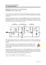
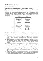
Nomenclature for a typical xy plot. Figure 5.1–1
Z.R.K
5-2 More? See pages 260-261.

The following MATLAB session plots y = 0.4 √1.8x for 0
≤ x ≤ 52, where y represents the height of a rocket
after launch, in miles, and x is the horizontal
(downrange) distance in miles.
>>x = [0:0.1:52];
>>y = 0.4*sqrt(1.8*x);
>>plot(x,y)
>>xlabel(‘Distance (miles)’)
>>ylabel(‘Height (miles)’)
>>title(‘Rocket Height as a ...
Function of Downrange Distance’)
The resulting plot is shown on the next slide.
5-3
Z.R.K

The autoscaling feature in MATLAB selects tick-mark
spacing. Figure 5.1–2
5-4
Z.R.K

The plot will appear in the Figure window. You can
obtain a hard copy of the plot in several ways:
1. Use the menu system. Select Print on the File
menu in the Figure window. Answer OK when you
are prompted to continue the printing process.
2. Type print at the command line. This command
sends the current plot directly to the printer.
3. Save the plot to a file to be printed later or
imported into another application such as a word
processor. You need to know something about
graphics file formats to use this file properly. See
the subsection Exporting Figures.
5-5
Z.R.K

When you have finished with the plot, close
the figure window by selecting Close from
the File menu in the figure window.
Note that using the Alt-Tab key combination in
Windows-based systems will return you to
the Command window without closing the
figure window.
If you do not close the window, it will not
reappear when a new plot command is
executed. However, the figure will still be
updated.
5-6
Z.R.K

Requirements for a Correct Plot
The following list describes the essential features of
any plot:
1. Each axis must be labeled with the name of the
quantity being plotted and its units! If two or more
quantities having different units are plotted (such
as when plotting both speed and distance versus
time), indicate the units in the axis label if there is
room, or in the legend or labels for each curve.
2. Each axis should have regularly spaced tick
marks at convenient intervals—not too sparse,
but not too dense—with a spacing that is easy to
interpret and interpolate. For example, use 0.1, 0.2,
and so on, rather than 0.13, 0.26, and so on.
Z.R.K
5-7 (continued …)

Requirements for a Correct Plot (continued)
3. If you are plotting more than one curve or
data set, label each on its plot or use a
legend to distinguish them.
4. If you are preparing multiple plots of a
similar type or if the axis labels cannot
convey enough information, use a title.
5. If you are plotting measured data, plot each
data point with a symbol such as a circle,
square, or cross (use the same symbol for
every point in the same data set). If there are
many data points, plot them using the dot
symbol.
5-8
Z.R.K
(continued …)

Requirements for a Correct Plot (continued)
6. Sometimes data symbols are connected by lines
to help the viewer visualize the data, especially if
there are few data points. However, connecting
the data points, especially with a solid line, might
be interpreted to imply knowledge of what occurs
between the data points. Thus you should be
careful to prevent such misinterpretation.
7. If you are plotting points generated by
evaluating a function (as opposed to measured
data), do not use a symbol to plot the points.
Instead, be sure to generate many points, and
connect the points with solid lines.
5-9
Z.R.K

The grid and axis Commands
The grid command displays gridlines at the tick
marks corresponding to the tick labels. Type grid
on to add gridlines; type grid off to stop plotting
gridlines. When used by itself, grid toggles this
feature on or off, but you might want to use grid on
and grid off to be sure.
You can use the axis command to override the
MATLAB selections for the axis limits. The basic
syntax is axis([xmin xmax ymin ymax]). This
command sets the scaling for the x- and y-axes to the
minimum and maximum values indicated. Note that,
unlike an array, this command does not use
commas to separate the values.
Z.R.K
5-10 More? See pages 264-265.

The effects of the axis and grid commands. Figure 5.1–3
5-11
Z.R.K

The plot(y) function plots the values in y versus the
indices. Figure 5.1–4.
x = 0.1+0.9j; n = [0:0.01:10]; y = x.^n;
plot(y), xlabel(‘Real’), ylabel(‘Imaginary’)
5-12
Z.R.K

The fplot command plots a function specified
as a string. Figure 5.1–5
>>f=‘cos(tan(x)) – tan(sin(x))’; fplot(f,[1 2])
5-13
Z.R.K

The function in Figure 5.1–5 generated with the plot
command, which gives more control than the fplot
command. Figure 5.1–6
>>x=[1:0.01:2]; y = cos(tan(x)) – tan(sin(x));
>>plot(x, y)
5-14
Z.R.K

Plotting Polynomials with the
polyval Function.
To plot the polynomial
3x 5 + 2x 4 – 100x 3 + 2x 2 – 7x + 90
over the range –6 ≤ x ≤ 6 with a spacing
of 0.01, you type
>>x = [-6:0.01:6];
>>p = [3,2,-100,2,-7,90];
>>grid on
>>plot(x,polyval(p,x)), ...
xlabel(’x’), ylabel(’p’)
5-15
Z.R.K
More? See page 268.

An example of a Figure window. Figure 5.1–7
5-16
Z.R.K

Saving Figures
To save a figure that can be opened in
subsequent MATLAB sessions, save it in a
figure file with the .fig file name extension.
To do this, select Save from the Figure
window File menu or click the Save button
(the disk icon) on the toolbar.
If this is the first time you are saving the file,
the Save As dialog box appears. Make sure
that the type is MATLAB Figure (*.fig).
Specify the name you want assigned to the
figure file. Click OK.
5-17
Z.R.K

Exporting Figures
To save the figure in a format that can be used by
another application, such as the standard graphics
file formats TIFF or EPS, perform these steps.
1. Select Export Setup from the File menu. This dialog
lets you specify options for the output file, such as
the figure size, fonts, line size and style, and output
format.
2. Select Export from the Export Setup dialog. A
standard Save As dialog appears.
3. Select the format from the list of formats in the Save
As type menu. This selects the format of the exported
file and adds the standard file name extension given
to files of that type.
4. Enter the name you want to give the file, less the
extension. Then click Save.
Z.R.K
5-18 More? See pages 270-271.

On Windows systems, you can also copy a
figure to the clipboard and then paste it
into another application (like Paint):
1. Select Copy Options from the Edit menu.
The Copying Options page of the
Preferences dialog box appears.
2. Complete the fields on the Copying
Options page and click OK.
3. Select Copy Figure from the Edit menu.
5-19
Z.R.K

5-20
Subplots
You can use the subplot command to obtain
several smaller “subplots” in the same figure.
The syntax is subplot(m,n,p). This
command divides the Figure window into an
array of rectangular panes with m rows and n
columns. The variable p tells MATLAB to place
the output of the plot command following the
subplot command into the p th pane.
For example, subplot(3,2,5) creates an array
of six panes, three panes deep and two panes
across, and directs the next plot to appear in the
fifth pane (in the bottom-left corner).
Z.R.K

5-21
The following script file created Figure 5.2–1,
which shows the plots of the functions
y = e -1.2x sin(10x + 5) for 0 ≤ x ≤ 5 and
y = |x 3 − 100| for −6 ≤ x ≤ 6.
x = [0:0.01:5];
y = exp(-1.2*x).*sin(10*x+5);
subplot(1,2,1)
plot(x,y),axis([0 5 -1 1])
x = [-6:0.01:6];
y = abs(x.^3-100);
subplot(1,2,2)
plot(x,y),axis([-6 6 0 350])
The figure is shown on the next slide.
Z.R.K

Application of the subplot command. Figure 5.2–1
Z.R.K
5-22 More on subplots? See page 271.

Data Markers and Line Types
To plot y versus x with a solid line and u versus
v with a dashed line, type plot(x,y,u,v,’--
’), where the symbols
’--’ represent a dashed line. Table 5.2–1 gives
the symbols for other line types.
To plot y versus x with asterisks (*) connected
with a dotted line, you must plot the data twice
by typing plot(x,y,’*’,x,y,’:’).
To plot y versus x with green asterisks (∗)
connected with a red dashed line, you must
plot the data twice by typing
plot(x,y,’g*’,x,y,’r--’).
5-23
Z.R.K

Data plotted using asterisks connected with a dotted line.
5-24
Z.R.K

Specifiers for data markers,
line types, and colors. Table 5.2–1
Data markers †
Line types
Colors
Dot (.)
Asterisk (*)
Cross (×)
Circle ( )
Plus sign (+)
Square ( )
Diamond ( )
Five-pointed star (w)
.
*
×
+
s
d
p
Solid line
Dashed line
Dash-dotted line
Dotted line
––
– –
– .
….
Black
Blue
Cyan
Green
Magenta
Red
White
Yellow
k
b
c
g
m
r
w
y
†
Other data markers are available. Search for “markers” in MATLAB
help.
5-25
Z.R.K

Use of data markers. Figure 5.2–2
Z.R.K
5-26 More? See pages 273-274.

Labeling Curves and Data legend
The legend command automatically obtains from the plot
the line type used for each data set and displays a sample of
this line type in the legend box next to the string you
selected. The following script file produced the plot in Figure
5.2–4.
x = [0:0.01:2];
y = sinh(x);
z = tanh(x);
plot(x,y,x,z,’--’),xlabel(’x’), ...
ylabel(’Hyperbolic Sine and ...
Tangent’),legend(’sinh(x)’,’tanh(x)’)
5-27
Z.R.K

Application of the legend command. Figure 5.2–4
5-28
Z.R.K

The gtext and text commands are also useful. Figure 5.2–5
Z.R.K
5-29 See page 276.

Graphical solution of equations: Circuit representation of a
power supply and a load. Figure 5.2–6
i 1 = 0.16 (e 0.12v2 – 1)
R 1 = 30 Ω, v 1 = +15V. & v 2 =(0 to 20)V
5-30
Z.R.K

Plot of the load line and the device curve for Previous
circuit. Figure 5.2–7
5-31
Z.R.K

Application of the hold command. Figure 5.2–8
Z.R.K
5-32 See page 279.

Why use log scales? Rectilinear scales cannot properly display
variations over wide ranges. Figure 5.3–1
>> x=[0:.01:100]; y=sqrt((100*(1-0.01*x.^2).^2+0.02*x.^2)...
./ ((1-x.^2).^2+0.1*x.^2)); plot(x,y)
5-33
Z.R.K

A loglog plot can display wide variations in data values.
Figure 5.3–2
Z.R.K
5-34 See page 282.

Logarithmic Plots
It is important to remember the following
points when using log scales:
1. You cannot plot negative numbers on a log
scale, because the logarithm of a negative
number is not defined as a real number.
2. You cannot plot the number 0 on a log
scale, because log 10 0 = ln 0 = -∞. You
must choose an appropriately small
number as the lower limit on the plot.
Z.R.K
5-35 (continued…)

Logarithmic Plots (continued)
5-36
3. The tick-mark labels on a log scale are the
actual values being plotted; they are not
the logarithms of the numbers.
For example, the range of x values in the plot
in Figure 5.3–2 is from 10 −2 = 0.01 to 10 2 =
100.
4. Gridlines and tick marks within a decade
are unevenly spaced. If 8 gridlines or tick
marks occur within the decade, they
correspond to values equal to 2, 3, 4, . . . , 8,
9 times the value represented by the first
gridline or tick mark of the decade.
Z.R.K
(continued…)

Logarithmic Plots (continued)
5. Equal distances on a log scale correspond to
multiplication by the same constant (as opposed
to addition of the same constant on a rectilinear
scale).
For example, all numbers that differ by a factor of 10
are separated by the same distance on a log
scale. That is, the distance between 0.3 and 3 is
the same as the distance between 30 and 300.
This separation is referred to as a decade or
cycle.
The plot shown in Figure 5.3–2 covers three
decades in x (from 0.01 to 100) and four decades
in y and is thus called a four-by-three-cycle plot.
5-37
Z.R.K

MATLAB has three commands for generating
plots having log scales. The appropriate
command depends on which axis must have a
log scale.
1. Use the loglog(x,y) command to
have both scales logarithmic.
2. Use the semilogx(x,y) command to
have the x scale logarithmic and the y scale
rectilinear.
3. Use the semilogy(x,y) command to
have the y scale logarithmic and the x scale
rectilinear.
5-38
Z.R.K

Two data sets plotted on four types of plots. Figure 5.3–3
5-39
Z.R.K
See page 285.

Application of logarithmic plots: An RC circuit.
Figure 5.3–4
v o /v i = (1 / | 1 + RCs |)
s = jw, Xc = 1/jwC, Xc = 1/sC .
5-40
Z.R.K

Frequency-response plot of a low-pass RC circuit.
Figure 5.3–5
5-41
Z.R.K
See pages 286-287.

Frequency-response plot of a low-pass RC circuit.
Z.R.K

Specialized plot commands. Table 5.3–1
Command
bar(x,y)
plotyy(x1,y1,x2,y2)
polar(theta,r,’type’)
stairs(x,y)
stem(x,y)
Description
Creates a bar chart of y versus x.
Produces a plot with two y-axes, y1
on the left and y2 on the right.
Produces a polar plot from the polar
coordinates theta and r, using the
line type, data marker, and colors
specified in the string type.
Produces a stairs plot of y versus x.
Produces a stem plot of y versus x.
5-43
Z.R.K

x = [0:pi/20:pi];
>> bar(x,sin(x))
5-44
Z.R.K

x = [0:pi/50:2*pi];
>> polar(x, sin(2*x)),grid
5-45
Z.R.K

x = [0:pi/20:2*pi];
>> stairs(x,sin(x)),grid;
>> axis([0 2*pi -1 1]);
5-46
Z.R.K

x = [-2*pi:pi/20:2*pi];
>> x = x + (~x)*eps; y=sin(pi*x)./(pi*x);
>> stem(x,y), axis([-2*pi 2*pi -.25 1])
5-47
Z.R.K

x = [-2*pi:pi/20:4*pi];
>> fill(x,sin(x),'c');
>> axis([0 4*pi -1 1])
5-48
Z.R.K

Interactive Plotting in MATLAB
This interface can be advantageous in
situations where:
• You need to create a large number of
different types of plots,
• You must construct plots involving many
data sets,
• You want to add annotations such as
rectangles and ellipses, or
• You want to change plot characteristics
such as tick spacing, fonts,
bolding, italics, and colors.
5-49
Z.R.K
More? See pages 292-298.

The interactive plotting environment in
MATLAB is a set of tools for:
• Creating different types of graphs,
• Selecting variables to plot directly from
the Workspace Browser,
• Creating and editing subplots,
• Adding annotations such as lines,
arrows, text, rectangles, and ellipses, and
• Editing properties of graphics objects,
such as their color, line weight, and font.
5-50
Z.R.K

The Figure window with the Figure toolbar displayed.
Figure 5.4–1
5-51
Z.R.K

The Figure window with the Figure and Plot Edit toolbars displayed.
Figure 5.4–2
5-52
Z.R.K

The Plot Tools interface includes the following
three panels associated with a given figure.
• The Figure Palette: Use this to create and
arrange subplots, to view and plot workspace
variables, and to add annotations.
• The Plot Browser: Use this to select and
control the visibility of the axes or graphics
objects plotted in the figure, and to add data for
plotting.
• The Property Editor: Use this to set basic
properties of the selected object and to obtain
access to all properties through the Property
Inspector.
5-53
Z.R.K

The Figure window with the Plot Tools activated. Figure 5.4–3
5-54
Z.R.K

The polyfit function is based on the
least-squares method. Its syntax is
p =
polyfit(x,y,n)
Fits a polynomial of degree n
to data described by the
vectors x and y, where x is
the independent
variable. Returns a row
vector p of length n+1 that
contains the polynomial
coefficients in order of
descending powers.
5-55
Z.R.K
See page 315, Table 5.6-1.

Three-Dimensional Line Plots plot3
The curve x = e -0.05t sin t, y = e -0.05t cos t, z
=tcan be plotted with the
plot3(x , y, z) function.
The following program uses the plot3 function to
generate the 3-D spiral curve shown in Figure 5.8–1.
>>t = [0:pi/50:10*pi];
>>plot3(exp(-0.05*t).*sin(t),...
exp(-0.05*t).*cos(t),t),...
xlabel(’x’),ylabel(’y’),zlabel(’z’),grid
5-56
Z.R.K

The curve x = e -0.05t sin t, y = e -0.05t cos t, z = t plotted with
the plot3(x , y, z) function. Figure 5.8–1
Z.R.K
5-57 More? See pages 334-335.

Surface Plots mesh:
The following session shows how to generate the
surface plot of the function
z = xe -[(x-y2 ) 2 +y 2 ] , for −2 ≤ x ≤ 2 and −2 ≤ y ≤ 2,
with a spacing of 0.1. This plot appears in Figure 5.8–
2.
>>[X,Y] = meshgrid(-2:0.1:2);
>>Z = X.*exp(-((X-Y.^2).^2+Y.^2));
>>mesh(X,Y,Z),xlabel(’x’), ...
ylabel(’y’), zlabel(’z’)
Z.R.K
5-58 See the next slide.

A plot of the surface z = xe -[(x-y2 ) 2 +y 2 ]
created with the mesh function. Figure 5.8–2
Z.R.K
5-59 More? See pages 335-336.

The following session generates the contour plot
of the function whose surface plot is shown in
Figure 5.8–2; namely, z = xe -[(x-y2 ) 2 +y 2 ] ,
for −2 ≤ x ≤ 2 and −2 ≤ y ≤ 2, with a spacing of
0.01. This plot appears in Figure 5.8–3.
>>[X,Y] = meshgrid(-2:0.1:2);
>>Z = X.*exp(-((X- Y.^2).^2+Y.^2));
>>contour(X,Y,Z),xlabel(’x’),ylabel(’y’)
5-60
Z.R.K

A contour plot of the surface z = xe -[(x-y2 ) 2 +y 2 ] created
with the contour function. Figure 5.8–3
Z.R.K
5-61 More? See page 337.

Three-dimensional plotting functions. Table 5.8–1
Function
Description
contour(x,y,z)
mesh(x,y,z)
meshc(x,y,z)
meshz(x,y,z)
surf(x,y,z)
surfc(x,y,z)
[X,Y] = meshgrid(x,y)
[X,Y] = meshgrid(x)
waterfall(x,y,z)
5-62
Creates a contour plot.
Creates a 3D mesh surface plot.
Same as mesh but draws contours under the
surface.
Same as mesh but draws vertical reference lines
under the surface.
Creates a shaded 3D mesh surface plot.
Same as surf but draws contours under the
surface.
Creates the matrices X and Y from the vectors x
and y to define a rectangular grid.
Same as [X,Y]= meshgrid(x,x).
Same as mesh but draws mesh lines in one
direction only.
Z.R.K

Plots of the surface z = xe -(x2 +y 2) created with the mesh
function and its variant forms: a) mesh, b) meshc,
c) meshz, and d) waterfall. Figure 5.8–4
5-63
Z.R.K

Example to plot 3D
5-64
If you want to see the famous Mexican hat
, type the following commands :
>> [x y] = meshgrid(-8:0.5:8);
>> r = sqrt(x.ˆ2 + y.ˆ2) + eps;
>> z = sin(r)./r;
>> mesh(z);
Why + eps ?
Try surf(z) to generate a faceted (tiled)
view of the surface.
Then try with surf(z) the shading
interp command.
Z.R.K

5-65
Famous Mexican
Z.R.K
hat.

5-66
Famous Mexican hat, with
meshgrid(-8:0.1:8) Z.R.K and surf(z)

5-67
Famous Mexican hat, with
meshgrid(-8:0.1:8),
Z.R.K
surf(z)and shading interp.

Visualizing vector fields
The function quiver draws little arrows to indicate a gradient
or other vector field. Although it produces a 2-D plot, it’s
often used in conjunction with contour. As an example,
consider the scalar function of two variables
V = x 2 + y. The gradient of V is defined as the vector field
∇V = ( ∂V / ∂x , ∂V / ∂y ) = (2x, 1).
The following statements draw arrows indicating the
direction of ∇V at points in the x-y plane (see the next figure).
[x y] = meshgrid(-2:.2:2, -2:.2:2);
V = x.^2 + y;
dx = 2*x;
dy = dx; % dy same size as dx
dy(:,:) = 1; % now dy is same size as dx but all 1’s
contour(x, y, V), hold on
quiver(x, y, dx, dy), hold off
5-68
Z.R.K

Gradients and level surfaces
Z.R.K

Example to plot 3D with surface and colormap:
See Primer in Matlab
figure(1) ; clf
t = linspace(0, 2*pi, 512);
[u,v] = meshgrid(t) ;
a = -0.2 ; b = .5 ; c = .1 ;
n = 2;
x = (a*(1-v/(2*pi)) .* (1+cos(u)) + c) .* cos(n*v);
y = (a*(1-v/(2*pi)) .* (1+cos(u)) + c) .* sin(n*v);
z = b*v/(2*pi) + a*(1-v/(2*pi)) .* sin(u);
surf(x,y,z,y)
shading interp
axis off
axis equal
colormap(hsv(1024))
material shiny
lighting gouraud
lightangle(80, -40)
lightangle(-90, 60)
view([-150 10])
5-70
Z.R.K

5-71
Z.R.K

End of Chapter 5
?
Problems Page 340 - 357 !
Solve: 3, 9, 11, 27, 35, 49, 52.
www.ju.edu.jo\zkhatib
Z.R.K
Z.R.J.K