Time Series - STAT - EPFL
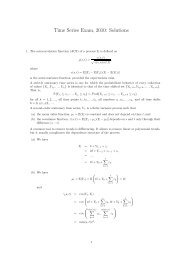
Time Series - STAT - EPFL
Time Series - STAT - EPFL

Create successful ePaper yourself
Turn your PDF publications into a flip-book with our unique Google optimized e-Paper software.
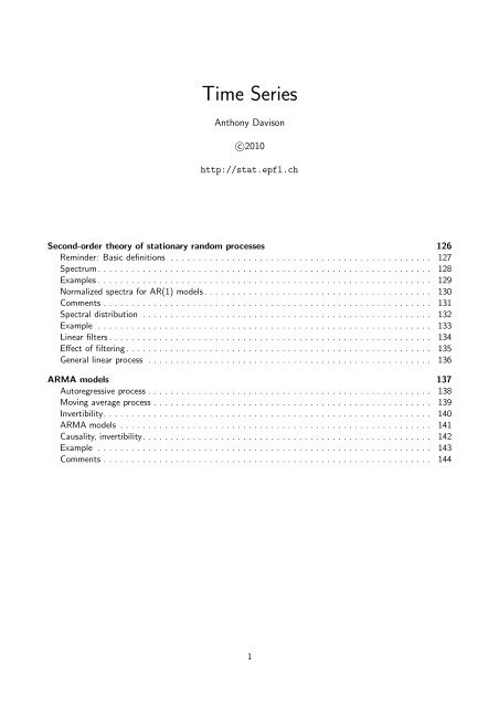
<strong>Time</strong> <strong>Series</strong><br />
Anthony Davison<br />
c○2010<br />
http://stat.epfl.ch<br />
Second-order theory of stationary random processes 126<br />
Reminder: Basic definitions . . . . . . . . . . . . . . . . . . . . . . . . . . . . . . . . . . . . . . . . . . . . . . . 127<br />
Spectrum. . . . . . . . . . . . . . . . . . . . . . . . . . . . . . . . . . . . . . . . . . . . . . . . . . . . . . . . . . . . 128<br />
Examples . . . . . . . . . . . . . . . . . . . . . . . . . . . . . . . . . . . . . . . . . . . . . . . . . . . . . . . . . . . . 129<br />
Normalized spectra for AR(1) models. . . . . . . . . . . . . . . . . . . . . . . . . . . . . . . . . . . . . . . . . 130<br />
Comments . . . . . . . . . . . . . . . . . . . . . . . . . . . . . . . . . . . . . . . . . . . . . . . . . . . . . . . . . . . 131<br />
Spectral distribution . . . . . . . . . . . . . . . . . . . . . . . . . . . . . . . . . . . . . . . . . . . . . . . . . . . . 132<br />
Example . . . . . . . . . . . . . . . . . . . . . . . . . . . . . . . . . . . . . . . . . . . . . . . . . . . . . . . . . . . . 133<br />
Linear filters . . . . . . . . . . . . . . . . . . . . . . . . . . . . . . . . . . . . . . . . . . . . . . . . . . . . . . . . . . 134<br />
Effect of filtering. . . . . . . . . . . . . . . . . . . . . . . . . . . . . . . . . . . . . . . . . . . . . . . . . . . . . . . 135<br />
General linear process . . . . . . . . . . . . . . . . . . . . . . . . . . . . . . . . . . . . . . . . . . . . . . . . . . . 136<br />
ARMA models 137<br />
Autoregressive process . . . . . . . . . . . . . . . . . . . . . . . . . . . . . . . . . . . . . . . . . . . . . . . . . . . 138<br />
Moving average process . . . . . . . . . . . . . . . . . . . . . . . . . . . . . . . . . . . . . . . . . . . . . . . . . . 139<br />
Invertibility. . . . . . . . . . . . . . . . . . . . . . . . . . . . . . . . . . . . . . . . . . . . . . . . . . . . . . . . . . . 140<br />
ARMA models . . . . . . . . . . . . . . . . . . . . . . . . . . . . . . . . . . . . . . . . . . . . . . . . . . . . . . . . 141<br />
Causality, invertibility. . . . . . . . . . . . . . . . . . . . . . . . . . . . . . . . . . . . . . . . . . . . . . . . . . . . 142<br />
Example . . . . . . . . . . . . . . . . . . . . . . . . . . . . . . . . . . . . . . . . . . . . . . . . . . . . . . . . . . . . 143<br />
Comments . . . . . . . . . . . . . . . . . . . . . . . . . . . . . . . . . . . . . . . . . . . . . . . . . . . . . . . . . . . 144<br />
1
Second-order theory of stationary random processes slide 126<br />
Reminder: Basic definitions<br />
Definition 28 (a) A random function is a set of random variables {Y (t)} such that the time-index t<br />
can take any real value.<br />
(b) The trend of {Y t } is the non-random function µ(t) = E{Y (t)}, and its autocovariance function<br />
is<br />
γ(t,s) = cov{Y (t),Y (s)} = E[{Y (t) − µ(t)}{Y (s) − µ(s)}], t,s ∈ R.<br />
The mean and covariance functions constitute the second-order properties of {Y (t)}. They<br />
determine the entire distribution of the random function if the joint distribution of any finite collection<br />
of random variables {Y (t 1 ),... ,Y (t k )} is multivariate normal.<br />
(c) The random function is stationary if µ(t) = µ and γ(t,s) = γ(|t − s|): the trend is constant and<br />
the covariance between Y (t) and Y (s) depends only on their time separation t − s. In this case we<br />
can define the autocorrelation function ρ(t) = γ(t,0)/γ(0,0).<br />
(d) A random sequence is a collection of random variables {Y t } in which the time index takes only<br />
integer values: t ∈ Z. We use a subscript notation to make this clear.<br />
(e) A white noise sequence is a random sequence consisting of mutually independent random<br />
variables each with mean zero and variance σ 2 .<br />
<strong>Time</strong> <strong>Series</strong> Spring 2010 – slide 127<br />
Spectrum<br />
Definition 29 (a) The autocovariance generating function of a stationary random sequence {Y t }<br />
with autocovariances γ k = cov(Y t ,Y t+k ) is<br />
(b) The spectrum of {Y t } is<br />
G(z) =<br />
∞∑<br />
k=−∞<br />
f(ω) = G(e −2πiω ) =<br />
γ k z k , z ∈ C.<br />
∞∑<br />
k=−∞<br />
γ k e −2πikω , ω ∈ R,<br />
where i 2 = −1; this may also be written as the real-valued function<br />
f(ω) = γ 0 + 2<br />
∞∑<br />
γ k cos(2πkω), ω ∈ R. (5)<br />
k=1<br />
The normalised spectrum is f ∗ (ω) = f(ω)/γ 0 .<br />
The spectrum provides a convenient summary of the second-order properties of the process in a single<br />
function, and also shows the effect of linear operations on the series very simply.<br />
<strong>Time</strong> <strong>Series</strong> Spring 2010 – slide 128<br />
127
Examples<br />
Example 30 Find the spectrum and normalised spectrum for white noise.<br />
Example 31 Show that the spectrum of the AR(1) process Y t = αY t−1 + ε t with |α| < 1 is<br />
and that the normalised spectrum is<br />
f(ω) =<br />
f ∗ (ω) =<br />
σ 2<br />
1 − 2α cos(2πω) + α 2,<br />
1 − α 2<br />
1 − 2α cos(2πω) + α 2.<br />
<strong>Time</strong> <strong>Series</strong> Spring 2010 – slide 129<br />
Normalized spectra for AR(1) models<br />
Y<br />
−4 −2 0 1 2 3<br />
Y<br />
−4 −2 0 1 2 3<br />
0 50<br />
alpha=−0.5<br />
100 150 200<br />
<strong>Time</strong><br />
alpha=0.5<br />
0 50 100 150 200<br />
<strong>Time</strong><br />
f*(w)<br />
0.5 1.0 1.5 2.0 2.5 3.0<br />
f*(w)<br />
0.5 1.0 1.5 2.0 2.5 3.0<br />
0.0 0.1 0.2 0.3 0.4 0.5<br />
w<br />
0.0 0.1 0.2 0.3 0.4 0.5<br />
w<br />
alpha=0.9<br />
Y<br />
−4 −2 0 2 4<br />
f*(w)<br />
0 5 10 15<br />
0 50 100 150 200 0.0 0.1 0.2 0.3 0.4 0.5<br />
<strong>Time</strong><br />
w<br />
<strong>Time</strong> <strong>Series</strong> Spring 2010 – slide 130<br />
128
Comments<br />
□ The form of the spectrum suggests that<br />
f(ω) = f(−ω), f(ω) = f(ω + k), k ∈ Z,<br />
so f need only be defined in 0 < ω < 1 2<br />
—recall the definition of the periodogram.<br />
□ The variance of the average Y of data Y 1 ,... ,Y n from a stationary process satisfies<br />
{<br />
lim nvar(Y ) = lim<br />
n→∞ n→∞<br />
}<br />
n−1<br />
∑<br />
∞∑<br />
γ 0 + 2 (1 − h/n)γ h = γ 0 + 2 γ h = f(0)<br />
h=1<br />
for large n. Thus the spectral density at the origin, if finite, equals the (rescaled) variance of Y .<br />
□ We easily see that ∫ 1/2<br />
−1/2 f(ω)dω = γ 0.<br />
□ The spectrum is the discrete Fourier transform of the autocovariance sequence.<br />
□ The inverse Fourier transform gives the autocovariance function by<br />
γ k =<br />
∫ 1/2<br />
−1/2<br />
e 2πikω f(ω)dω = 2<br />
∫ 1/2<br />
□ The spectral density need not always exist; cf. Example 33.<br />
0<br />
h=1<br />
cos(2πkω)f(ω)dω, k ∈ Z. (6)<br />
<strong>Time</strong> <strong>Series</strong> Spring 2010 – slide 131<br />
Spectral distribution<br />
Theorem 32 (a) A set of numbers {γ h } h∈Z is the autocovariance function of a stationary random<br />
sequence iff there exists a unique bounded function F defined on [− 1 2 , 1 2<br />
] such that F(−1/2) = 0, F<br />
is right-continuous and non-decreasing, with symmetric increments about zero, and<br />
∫<br />
γ h = e 2πihu dF(u), h ∈ Z.<br />
(−1/2,1/2]<br />
The function F is called the spectral distribution function of γ h , and its derivative, if it exists, is<br />
called the spectral density function, or spectrum.<br />
(b) If ∑ h |γ h| < ∞, then f exists.<br />
(c) A function f(ω) defined on [−1/2,1/2] is the spectrum of a stationary process if and only if<br />
f(ω) = f(−ω), f(ω) ≥ 0, and ∫ 1/2<br />
−1/2<br />
f(ω)dω < ∞.<br />
□ The symmetric increments property means that if 0 ≤ a < b ≤ 1 2 , then<br />
F(b) − F(a) = F(−a) − F(−b).<br />
□ The interpretation of F is that F(ω 2 ) − F(ω 1 ) measures the variation accounted for by<br />
fluctuations in frequency in the interval (ω 1 ,ω 2 ).<br />
□ Part (c) of the theorem suggests how we may construct covariance functions with desired<br />
properties, by choosing an appropriate spectrum—note that f may be any scaled density function.<br />
<strong>Time</strong> <strong>Series</strong> Spring 2010 – slide 132<br />
129
Example<br />
Example 33 Show that the covariance function of the stationary random sequence given by<br />
Y t = U 1 cos(2πω 0 t) + U 2 sin(2πω 0 t),<br />
U 1 ,U 2<br />
iid ∼ N(0,σ 2 ),<br />
may be written as<br />
γ h =<br />
∫ 1/2<br />
−1/2<br />
⎧<br />
⎪⎨ 0, ω < −ω 0 ,<br />
e 2πiωh dF(ω), F(ω) = σ<br />
⎪⎩<br />
2 /2, −ω 0 ≤ ω < ω 0 ,<br />
σ 2 , ω 0 ≤ ω.<br />
<strong>Time</strong> <strong>Series</strong> Spring 2010 – slide 133<br />
Linear filters<br />
Definition 34 A linear filter is a transformation of the random sequence {U t } of the form<br />
Y t =<br />
∞∑<br />
j=−∞<br />
□ If {U t } is stationary and<br />
a j U t−j . (7)<br />
– only a finite number of the a j are non-zero, then {Y t } is stationary;<br />
– infinitely many of the a j are non-zero, then the properties of {Y t } depend on their values.<br />
□ The relation between the spectra of the sequences is given by the following theorem:<br />
Theorem 35 The spectra of two stationary random sequences {U t } and {Y t } satisfying (7) are<br />
related by<br />
f Y (ω) = |a(ω)| 2 f U (ω),<br />
where a(ω) = ∑ ∞<br />
j=−∞ a je −2πijω is the transfer function of the linear filter.<br />
<strong>Time</strong> <strong>Series</strong> Spring 2010 – slide 134<br />
Effect of filtering<br />
Example 36 Find the spectrum of a three-point moving average of an AR(1) process.<br />
Spectrum<br />
Squared modulus of transfer function<br />
Filtered spectrum<br />
f(w)<br />
0 1 2 3 4<br />
|a(w)|^2<br />
0.0 0.2 0.4 0.6 0.8 1.0<br />
f(w)|a(w)|^2<br />
0.0 0.1 0.2 0.3 0.4<br />
0.0 0.1 0.2 0.3 0.4 0.5 0.0 0.1 0.2 0.3 0.4 0.5 0.0 0.1 0.2 0.3 0.4 0.5<br />
w<br />
w<br />
w<br />
<strong>Time</strong> <strong>Series</strong> Spring 2010 – slide 135<br />
130
General linear process<br />
Theorem 37 The spectrum of the general linear process<br />
Y t =<br />
∞∑<br />
a j ε t−j , (8)<br />
j=0<br />
where {ε t } is white noise, may be written as<br />
f(ω) = b 0 +<br />
∞∑<br />
b m cos(2πmω), −1/2 ≤ ω ≤ 1/2. (9)<br />
m=1<br />
□ Any real-valued even continuous function that satisfies f(ω) = f(ω + k) for integer k can be<br />
expressed as the (implicit) Fourier series (9), so any stationary random sequence with a<br />
continuous spectrum can be represented as a general linear process—at least so far as<br />
second-order properties are concerned.<br />
□ The general linear representation (8) is only useful if it involves only a few parameters—hence the<br />
use of ARMA models, which are quite flexible linear models with finite parameters.<br />
□ The computations leading to (9) implicitly presuppose that ∑ a 2 j < ∞, which then implies that<br />
{Y t } is stationary with finite variance and covariance function.<br />
<strong>Time</strong> <strong>Series</strong> Spring 2010 – slide 136<br />
ARMA models slide 137<br />
Autoregressive process<br />
Definition 38 An autoregressive process of order p, AR(p), model, is of the form<br />
Y t = φ 1 Y t−1 + φ 2 Y t−2 + · · · + φ p Y t−p + ε t , (10)<br />
where {Y t } is stationary and φ 1 ,... ,φ p are constants and φ p ≠ 0. Unless otherwise mentioned, we<br />
iid<br />
assume here that ε t ∼ N(0,σ 2 ). A process with non-zero mean is obtained by replacing Y t in (10) by<br />
Y t − µ, etc.<br />
The backshift operator B can be used to write (10) in the form<br />
(1 − φ 1 B − · · · − φ p B p )Y t = φ(B)Y t = ε t ,<br />
where φ(B) is the autoregressive operator, and this suggests writing<br />
Y t = φ(B) −1 ε t<br />
to get the causal representation Y t = ∑ ∞<br />
j=0 ψ jε t−j = ψ(B)ε t , if it exists. To find the coefficients of<br />
ψ(B), we suppose that such a representation exists, and then match terms on the left and right of the<br />
equation φ(B)Y t = φ(B)ψ(B)ε t = ε t .<br />
<strong>Time</strong> <strong>Series</strong> Spring 2010 – slide 138<br />
131
Moving average process<br />
Definition 39 A moving average model of order q, MA(q), is of the form<br />
Y t = ε t + θ 1 ε t−1 + · · · + θ q ε t−q , (11)<br />
where θ 1 ,... ,θ q are constants, θ q ≠ 0, and ε t<br />
iid ∼ N(0,σ 2 ). A process with non-zero mean is obtained<br />
by replacing Y t in (11) by Y t − µ.<br />
The backshift operator B can be used to write (11) in the form<br />
Y t = (1 + θ 1 B + · · · + θ q B q )ε t = θ(B)ε t ,<br />
where θ(B) is the moving average operator. The process (11) is stationary for any values of the θ r .<br />
Example 40 Show that the MA(1) processes with parameters θ 1 and 1/θ 1 are statistically<br />
indistinguishable.<br />
<strong>Time</strong> <strong>Series</strong> Spring 2010 – slide 139<br />
Invertibility<br />
Definition 41 A moving average process {Y t } is called invertible if it has an infinite autoregressive<br />
representation<br />
∞∑<br />
ε t = a j Y t−j .<br />
□ This definition is needed simply in order to ensure the identifiability of MA processes.<br />
□ In Example 40 it is easy to check which version is invertible, we write<br />
ε t = (1 + θ 1 B) −1 Y t =<br />
which is convergent iff |θ 1 | < 1.<br />
j=0<br />
∞∑<br />
∞∑<br />
(−θ 1 B) j Y t = (−θ 1 ) j Y t−j ,<br />
j=0<br />
<strong>Time</strong> <strong>Series</strong> Spring 2010 – slide 140<br />
j=0<br />
132
ARMA models<br />
Definition 42 A time series {Y t } is an autoregressive-moving average process of order p,q,<br />
ARMA(p,q), model, if it is stationary and of the form<br />
Y t = φ 1 Y t−1 + φ 2 Y t−2 + · · · + φ p Y t−p + ε t + θ 1 ε t−1 + · · · + θ q ε t−q , (12)<br />
where φ 1 ,...,φ p ,θ 1 ,... ,θ q are constants with φ p ,θ q ≠ 0. Unless otherwise mentioned, we assume<br />
iid<br />
that ε t ∼ N(0,σ 2 ). A process with non-zero mean is obtained by replacing the Y s in (12) by Y t − µ,<br />
etc.<br />
□ We use the autoregressive and moving average operators to write (12) as<br />
φ(B)Y t = θ(B)ε t .<br />
The properties of the process are intimately tied to the polynomials φ(z),θ(z), where we take<br />
z ∈ C. Let D = {z ∈ C : |z| ≤ 1} denote the unit disk in the complex plane.<br />
□ We remove common factors from φ(B) and θ(B) to eliminate overparametrisation, also called<br />
parameter redundancy.<br />
<strong>Time</strong> <strong>Series</strong> Spring 2010 – slide 141<br />
Causality, invertibility<br />
Definition 43 An ARMA(p,q) process φ(B)Y t = θ(B)ε t is causal if it can be written as a linear<br />
process<br />
∞∑<br />
Y t = ψ j ε t−j = ψ(B)ε t ,<br />
where ∑ |ψ j | < ∞, and we set ψ 0 = 1. It is invertible if it can be written as<br />
where ∑ |π j | < ∞, and we set π 0 = 1,<br />
ε t =<br />
j=0<br />
∞∑<br />
π j Y t−j = π(B)Y t ,<br />
j=0<br />
Theorem 44 (a) An ARMA(p,q) process φ(B)Y t = θ(B)ε t is causal iff φ(z) ≠ 0 within D. If so,<br />
then the coefficients of ψ(z) satisfy ψ(z) = θ(z)/φ(z) for z ∈ D.<br />
(b) The process is invertible iff θ(z) ≠ 0 for z ∈ D. If so, then the coefficients of π(z) satisfy<br />
π(z) = φ(z)/θ(z) for for z ∈ D.<br />
Thus the process is causal iff the roots of φ(z) lie outside D, and invertible iff the roots of θ(z) lie<br />
outside D.<br />
<strong>Time</strong> <strong>Series</strong> Spring 2010 – slide 142<br />
Example<br />
Example 45 Investigate the properties of the process<br />
Y t = 0.4Y t−1 + 0.45Y t−2 + ε t + ε t−1 + 0.25ε t−2 .<br />
<strong>Time</strong> <strong>Series</strong> Spring 2010 – slide 143<br />
133
Comments<br />
□ Why use ARMA processes<br />
– usually an empirical model, using φ 1 ,...φ p ,θ 1 ,...,θ q as summary statistics, but with no<br />
implication that the model has a ‘scientific’, explanatory, basis in terms of the underlying data<br />
generating mechanism<br />
– the spectrum of an ARMA process can take many forms without p or q being very large, so<br />
they provide a flexible and parsimonious way to approximate a wide range of second-order<br />
properties<br />
– they are useful for forecasting, or for other settings where the autocorrelation structure of the<br />
data is not of primary interest<br />
□ ARMA models are not usually useful when the focus is on understanding the underlying<br />
mechanism that generates the data<br />
□ AR and MA models separately may provide more interpretable models in such cases:<br />
– AR models have Markov structure, which may be interpretable<br />
– MA models stem from weighted moving averages, which may be interpretable<br />
<strong>Time</strong> <strong>Series</strong> Spring 2010 – slide 144<br />
134