Time Series - STAT - EPFL

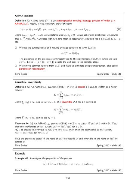
ARMA models
Definition 42 A time series {Y t } is an autoregressive-moving average process of order p,q,
ARMA(p,q), model, if it is stationary and of the form
Y t = φ 1 Y t−1 + φ 2 Y t−2 + · · · + φ p Y t−p + ε t + θ 1 ε t−1 + · · · + θ q ε t−q , (12)
where φ 1 ,...,φ p ,θ 1 ,... ,θ q are constants with φ p ,θ q ≠ 0. Unless otherwise mentioned, we assume
iid
that ε t ∼ N(0,σ 2 ). A process with non-zero mean is obtained by replacing the Y s in (12) by Y t − µ,
etc.
□ We use the autoregressive and moving average operators to write (12) as
φ(B)Y t = θ(B)ε t .
The properties of the process are intimately tied to the polynomials φ(z),θ(z), where we take
z ∈ C. Let D = {z ∈ C : |z| ≤ 1} denote the unit disk in the complex plane.
□ We remove common factors from φ(B) and θ(B) to eliminate overparametrisation, also called
parameter redundancy.
Time Series Spring 2010 – slide 141
Causality, invertibility
Definition 43 An ARMA(p,q) process φ(B)Y t = θ(B)ε t is causal if it can be written as a linear
process
∞∑
Y t = ψ j ε t−j = ψ(B)ε t ,
where ∑ |ψ j | < ∞, and we set ψ 0 = 1. It is invertible if it can be written as
where ∑ |π j | < ∞, and we set π 0 = 1,
ε t =
j=0
∞∑
π j Y t−j = π(B)Y t ,
j=0
Theorem 44 (a) An ARMA(p,q) process φ(B)Y t = θ(B)ε t is causal iff φ(z) ≠ 0 within D. If so,
then the coefficients of ψ(z) satisfy ψ(z) = θ(z)/φ(z) for z ∈ D.
(b) The process is invertible iff θ(z) ≠ 0 for z ∈ D. If so, then the coefficients of π(z) satisfy
π(z) = φ(z)/θ(z) for for z ∈ D.
Thus the process is causal iff the roots of φ(z) lie outside D, and invertible iff the roots of θ(z) lie
outside D.
Time Series Spring 2010 – slide 142
Example
Example 45 Investigate the properties of the process
Y t = 0.4Y t−1 + 0.45Y t−2 + ε t + ε t−1 + 0.25ε t−2 .
Time Series Spring 2010 – slide 143
133