Time Series - STAT - EPFL

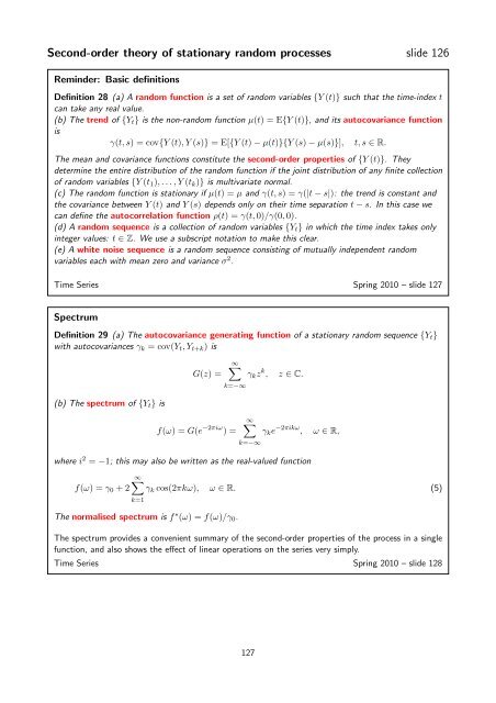
Second-order theory of stationary random processes slide 126
Reminder: Basic definitions
Definition 28 (a) A random function is a set of random variables {Y (t)} such that the time-index t
can take any real value.
(b) The trend of {Y t } is the non-random function µ(t) = E{Y (t)}, and its autocovariance function
is
γ(t,s) = cov{Y (t),Y (s)} = E[{Y (t) − µ(t)}{Y (s) − µ(s)}], t,s ∈ R.
The mean and covariance functions constitute the second-order properties of {Y (t)}. They
determine the entire distribution of the random function if the joint distribution of any finite collection
of random variables {Y (t 1 ),... ,Y (t k )} is multivariate normal.
(c) The random function is stationary if µ(t) = µ and γ(t,s) = γ(|t − s|): the trend is constant and
the covariance between Y (t) and Y (s) depends only on their time separation t − s. In this case we
can define the autocorrelation function ρ(t) = γ(t,0)/γ(0,0).
(d) A random sequence is a collection of random variables {Y t } in which the time index takes only
integer values: t ∈ Z. We use a subscript notation to make this clear.
(e) A white noise sequence is a random sequence consisting of mutually independent random
variables each with mean zero and variance σ 2 .
Time Series Spring 2010 – slide 127
Spectrum
Definition 29 (a) The autocovariance generating function of a stationary random sequence {Y t }
with autocovariances γ k = cov(Y t ,Y t+k ) is
(b) The spectrum of {Y t } is
G(z) =
∞∑
k=−∞
f(ω) = G(e −2πiω ) =
γ k z k , z ∈ C.
∞∑
k=−∞
γ k e −2πikω , ω ∈ R,
where i 2 = −1; this may also be written as the real-valued function
f(ω) = γ 0 + 2
∞∑
γ k cos(2πkω), ω ∈ R. (5)
k=1
The normalised spectrum is f ∗ (ω) = f(ω)/γ 0 .
The spectrum provides a convenient summary of the second-order properties of the process in a single
function, and also shows the effect of linear operations on the series very simply.
Time Series Spring 2010 – slide 128
127