Time Series - STAT - EPFL
Time Series - STAT - EPFL
Time Series - STAT - EPFL

You also want an ePaper? Increase the reach of your titles
YUMPU automatically turns print PDFs into web optimized ePapers that Google loves.
Example<br />
Example 33 Show that the covariance function of the stationary random sequence given by<br />
Y t = U 1 cos(2πω 0 t) + U 2 sin(2πω 0 t),<br />
U 1 ,U 2<br />
iid ∼ N(0,σ 2 ),<br />
may be written as<br />
γ h =<br />
∫ 1/2<br />
−1/2<br />
⎧<br />
⎪⎨ 0, ω < −ω 0 ,<br />
e 2πiωh dF(ω), F(ω) = σ<br />
⎪⎩<br />
2 /2, −ω 0 ≤ ω < ω 0 ,<br />
σ 2 , ω 0 ≤ ω.<br />
<strong>Time</strong> <strong>Series</strong> Spring 2010 – slide 133<br />
Linear filters<br />
Definition 34 A linear filter is a transformation of the random sequence {U t } of the form<br />
Y t =<br />
∞∑<br />
j=−∞<br />
□ If {U t } is stationary and<br />
a j U t−j . (7)<br />
– only a finite number of the a j are non-zero, then {Y t } is stationary;<br />
– infinitely many of the a j are non-zero, then the properties of {Y t } depend on their values.<br />
□ The relation between the spectra of the sequences is given by the following theorem:<br />
Theorem 35 The spectra of two stationary random sequences {U t } and {Y t } satisfying (7) are<br />
related by<br />
f Y (ω) = |a(ω)| 2 f U (ω),<br />
where a(ω) = ∑ ∞<br />
j=−∞ a je −2πijω is the transfer function of the linear filter.<br />
<strong>Time</strong> <strong>Series</strong> Spring 2010 – slide 134<br />
Effect of filtering<br />
Example 36 Find the spectrum of a three-point moving average of an AR(1) process.<br />
Spectrum<br />
Squared modulus of transfer function<br />
Filtered spectrum<br />
f(w)<br />
0 1 2 3 4<br />
|a(w)|^2<br />
0.0 0.2 0.4 0.6 0.8 1.0<br />
f(w)|a(w)|^2<br />
0.0 0.1 0.2 0.3 0.4<br />
0.0 0.1 0.2 0.3 0.4 0.5 0.0 0.1 0.2 0.3 0.4 0.5 0.0 0.1 0.2 0.3 0.4 0.5<br />
w<br />
w<br />
w<br />
<strong>Time</strong> <strong>Series</strong> Spring 2010 – slide 135<br />
130