Does Tail Dependence Make A Difference In the ... - Boston College

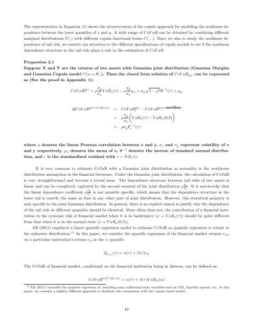
The representation in Equation (1) shows the attractiveness of the copula approach for modeling the nonlinear dependence
between the lower quantiles of x and y. A wide range of CoV aR can be obtained by combining different
marginal distributions F (.) with different copula functional forms C(., .). Since we aim to study the nonlinear dependence
of tail risk, we restrict our attention to the different specifications of copula models to see if the nonlinear
dependence structure in the tail risk plays a role in the estimation of CoV aR.
Propostion 2.1
Suppose X and Y are the returns of two assets with Gaussian joint distribution (Gaussian Margins
and Gaussian Copula model C(u, v; θ) ). Then the closed form solution of CoV aR y|x can be expressed
as (See the proof in Appendix 1):
CoV aR y|x
τ
= ρ σ y
σ x
V aR x (τ) − ρ σ y
σ x
µ x + σ y
√
1 − ρ2 Φ −1 (τ) + µ y
∆CoV aR y|x=V aRx(τ) = CoV aRτ
y|x − CoV aR y|x=median
= ρ σ (
)
y
V aR x (τ) − V aR x (0.5)
σ x
= ρσ y Fɛ
−1 (τ)
where ρ denotes the linear Pearson correlation between x and y, σ x and σ y represent volatility of x
and y respectively, µ x denotes the mean of x, Φ −1 denotes the inverse of standard normal distribution,
and ɛ is the standardized residual with ɛ ∼ N(0, 1).
It is very common to estimate CoVaR with a Gaussian joint distribution as normality is the workhorse
distribution assumption in the financial literature. Under the Gaussian joint distribution, the calculation of CoVaR
is very straightforward and become a trivial issue. The dependence structure between tail risks of two assets is
linear and can be completely captured by the second moment of the joint distribution ρ σy
σ x
. It is noteworthy that
the linear dependence coefficient ρ σy
σ x
is not quantile specific, which means that the dependence structure in the
lower tail is exactly the same as that in any other part of joint distribution. However, this statistical property is
only specific to the joint Gaussian distribution. In general, there is no explicit reason to justify why the dependence
of the tail risk at different quantiles should be identical. More often than not, the contribution of a financial institution
to the systemic risk of financial market when it is in bankruptcy (x = V aR x (τ)) should be quite different
from that when it is in the normal state (x = V aR x (0.5)).
AB (2011) employed a linear quantile regression model to estimate CoVaR as quantile regression is robust to
the unknown distribution. 11 In this paper, we consider the quantile regression of the financial market returns r mt
on a particular institution’s return r it at the α quantile
Q rmt (τ) = α(τ) + β(τ)r it
The CoVaR of financial market, conditional on the financial institution being in distress, can be defined as:
CoV aR m|V aRit(α) = α(τ) + β(τ)V aR it (α)
11 AB (2011) extended the quantile regression by including some additional state variables such as VIX, liquidity spread, etc. In this
paper, we consider a slightly different approach to facilitate the comparison with the copula based model.
10