Does Tail Dependence Make A Difference In the ... - Boston College

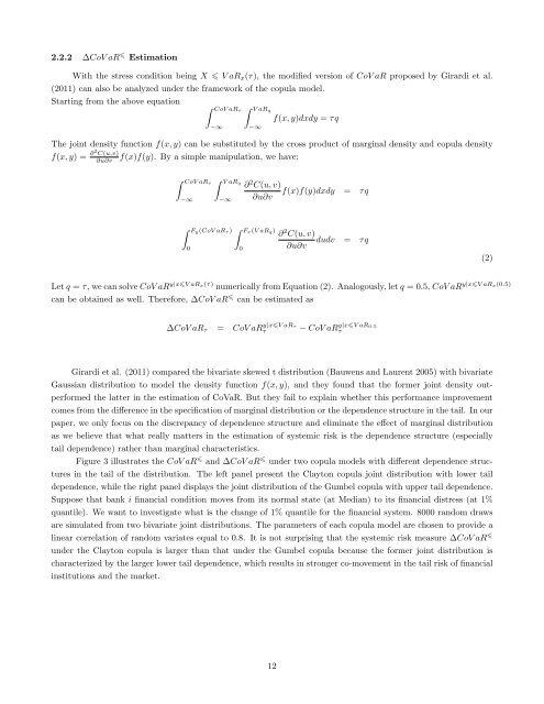
2.2.2 ∆CoV aR Estimation
With the stress condition being X V aR x (τ), the modified version of CoV aR proposed by Girardi et al.
(2011) can also be analyzed under the framework of the copula model.
Starting from the above equation
∫ CoV aRτ ∫ V aRq
−∞
−∞
f(x, y)dxdy = τq
The joint density function f(x, y) can be substituted by the cross product of marginal density and copula density
f(x, y) = ∂2 C(u,v)
∂u∂v
f(x)f(y). By a simple manipulation, we have:
∫ CoV aRτ ∫ V aRq
−∞ −∞
∂ 2 C(u, v)
f(x)f(y)dxdy = τq
∂u∂v
∫ Fy(CoV aR τ ) ∫ Fx(V aR q)
0
0
∂ 2 C(u, v)
dudv = τq
∂u∂v
(2)
Let q = τ, we can solve CoV aR y|xV aRx(τ) y|xV aRx(0.5)
numerically from Equation (2). Analogously, let q = 0.5, CoV aR
can be obtained as well. Therefore, ∆CoV aR can be estimated as
y|xV aRτ
∆CoV aR τ = CoV aRτ
y|xV aR0.5
− CoV aRτ
Girardi et al. (2011) compared the bivariate skewed t distribution (Bauwens and Laurent 2005) with bivariate
Gaussian distribution to model the density function f(x, y), and they found that the former joint density outperformed
the latter in the estimation of CoVaR. But they fail to explain whether this performance improvement
comes from the difference in the specification of marginal distribution or the dependence structure in the tail. In our
paper, we only focus on the discrepancy of dependence structure and eliminate the effect of marginal distribution
as we believe that what really matters in the estimation of systemic risk is the dependence structure (especially
tail dependence) rather than marginal characteristics.
Figure 3 illustrates the CoV aR and ∆CoV aR under two copula models with different dependence structures
in the tail of the distribution. The left panel present the Clayton copula joint distribution with lower tail
dependence, while the right panel displays the joint distribution of the Gumbel copula with upper tail dependence.
Suppose that bank i financial condition moves from its normal state (at Median) to its financial distress (at 1%
quantile). We want to investigate what is the change of 1% quantile for the financial system. 8000 random draws
are simulated from two bivariate joint distributions. The parameters of each copula model are chosen to provide a
linear correlation of random variates equal to 0.8. It is not surprising that the systemic risk measure ∆CoV aR
under the Clayton copula is larger than that under the Gumbel copula because the former joint distribution is
characterized by the larger lower tail dependence, which results in stronger co-movement in the tail risk of financial
institutions and the market.
12