Low-bond axisymmetric drop shape analysis for surface tension ...

More documents

Recommendations

Info

A.F. Stalder et al. / Colloids and Surfaces A: Physicochem. Eng. Aspects 364 (2010) 72–81 77 fore be considered as “classical” approaches in the light of works by Bashforth and Adams [9]. Among other values, all algorithms output contact angle, drop volume and surface tension being represented by either capillary constant c = · g/ or Bond parameter ˇ = · g · b 2 /. Each drop picture is analysed independently using the commercial programs and a manual specification of the drop base line is followed by the contour fit. The first algorithm – being called “SCA20” hereafter – is developed by DataPhysics in Germany [31] and offers support for communication with contact angle measuring devices sold by the company. The second algorithm will be named “ADSA” in the further course of this article and originates from the University of Toronto. It looks for a black drop on a white background wherefore greyscale values of obtained images need to be inverted prior to analysis (see Figs. 5 and 7). Applications and discussions of this code can frequently be found in literature [12,11,27,32,33]. Like with LBADSA, surface tension data needs to be calculated from capillary constant c or Bond parameter ˇ when using the commercial codes. 2.8. Processing of calculation results Due to some aberrant measurements, three filters needed to be introduced in order to check outputted datasets of all three algorithms for physical plausibility. The first such threshold restricts the contact angle to the range between 0 ◦ and 180 ◦ . Secondly, the capillary constant is constrained to positive values which assures c /= 0 for a correct calculation of surface tension. Thirdly, values for are limited to the interval of 0 mN/m to 1500 mN/m complying with literature specifications for coal ash slags [34–36,28,37]. Datasets are discarded completely if one of the presented filter conditions fails. In order to obtain surface tension values from output data, capillary constant c and drop volume v have to be used. By dividing an average sample mass ¯m determined before and after the experiment by the calculated drop volume, surface tension is derived according to = ¯m · g/v · c. It has to be noted that the density of the surrounding gas atmosphere is neglected in this approach. In addition, errors in drop volume calculation and mass determination directly affect the resulting surface tensions. This article solely presents data points that successfully passed the filter conditions for all three algorithms. 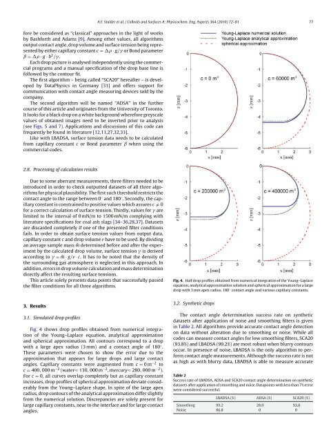Fig. 4. Half drop profiles obtained from numerical integration of the Young–Laplace equation, analytical approximation solution and spherical approximation for a large drop with 3 mm apex radius, 180 ◦ contact angle and various capillary constants. 3. Results 3.1. Simulated drop profiles Fig. 4 shows drop profiles obtained from numerical integration of the Young–Laplace equation, analytical approximation and spherical approximation. All contours correspond to a drop with a large apex radius (3 mm) and a contact angle of 180 ◦ . These parameters were chosen to show the error due to the approximation that appears for large drops and large contact angles. Capillary constants were augmented from c = 0m −2 to c = 400, 000 m −2 (water≈ 130, 000 m −2 , mercury≈ 280, 000 m −2 ). For c = 0, all curves overlap completely but as capillary constant increases, drop profiles of spherical approximation deviate considerably from the Young–Laplace shape. In spite of the large apex radius, drop contours of the analytical approximation differ slightly from the numerical solution. Discrepancies are solely present for large capillary constants, near to the interface and for large contact angles. 3.2. Synthetic drops The contact angle determination success rate on synthetic datasets after application of noise and smoothing filters is given in Table 2. All algorithms provide accurate contact angle detection on data without alteration due to smoothing or noise. While all codes can measure contact angles for low smoothing filters, SCA20 (93.8%) and LBADSA (99.2%) are most robust when blurry contours occur. In presence of noise, LBADSA is the only algorithm to perform contact angle measurements. Although the success rate is not as high as with blurry data, LBADSA is able to measure accurate Table 2 Success rate of LBADSA, ADSA and SCA20 contact angle determination on synthetic datasets after application of smoothing and noise. Datapoints with less than 7% error were considered successful. LBADSA (%) ADSA (%) SCA20 (%) Smoothing 99.2 28.0 93.8 Noise 86.8 0 0
78 A.F. Stalder et al. / Colloids and Surfaces A: Physicochem. Eng. Aspects 364 (2010) 72–81 Table 3 Ratio of plausible datapoints measured by LBADSA, ADSA and SCA20 in Figs. 5–7. A ratio of plausible datapoints below 100% indicate that in some situations either the algorithm failed to produce any result or that the result was aberant and excluded by the plausibility filter. LBADSA (%) ADSA (%) SCA20 (%) Serie from Fig. 5 91.0 86.5 59.5 Serie from Fig. 7 99.0 71.8 99.0 Serie from Fig. 6 89.8 6.8 98.3 Fig. 5. German black coal ash on graphite at 1310 ◦ C. Fig. 6. NaCl on graphite at 860 ◦ C. contact angles in 86.8% of the trials. In all cases, accuracy of contact angle measurements decreased as the smoothing or noise filter’s intensity increased. 3.3. Experimental drops During sessile drop measurements, mainly two different drop types were observed. Depending on substrate material, surrounding gas atmosphere and ash under investigation, upright round drops (Figs. 5 and 6) or flat drops (Fig. 7) can be found. The applied algorithms generally perform better on large round drops, yielding low-scattering surface tension values as a function of temperature. This finding is in full accordance with literature [27]. The ratio of plausible datapoints produced by the three algorithms is shown in Table 3. Unlike Table 2, Table 3 does not indicate the accuracy of the measurements but only the ability of each algorithm to measure data that are not aberrant. The plausible datapoints include all the measurements that could actually be performed by one algorithm (some images can make one algorithm fail and produce no measurements) and that were not excluded by the plausibility filter. While ADSA and SCA20 presented a wide range of ratio of plausible datapoints on different datasets (from 6.8% to 99.0%), LBADSA coherently presented a high ratio of plausible datapoints (≥89.8%). Nevertheless, Table 3 is not enough to assess the accuracy of the algorithms as one algorithm may gives out plausible yet inaccurate values. To underline previous statements, Fig. 8 provides calculated contact angle and surface tension data for a coal ash forming a round drop. Fig. 9 illustrates results for the image series of a flat drop in contrast. Whereas surface tension scatters far less when round drops are investigated, contact angle calculation exhibits an opposite trend. Analysis of the flat drop image series leads to nearly constant contact angle gradients for all three computer codes. While the ADSA algorithm yields equally smooth contact angle curves for round drops, LBADSA and SCA20 show scattering results in those cases. This is likely due to the detection of the drop baseline. While ADSA and SCA20 are not able to detect the interface by themselves and use a constant level (manually defined) instead, LBADSA automatically detects the baseline in every image. Common for nearly all round-drop-forming ashes are negative surface tension gradients at low temperatures and slightly rising or stagnating surface tensions at high temperatures (with respect to ADSA and LBADSA data). The increase of surface tension as well as the order of magnitude of surface tension values are in accordance with literature [34–36,28,37]. From Fig. 8 it is obvious that SCA20 outputs most deviating results whereas ADSA and LBADSA are in very good agreement with each other regarding surface tension. In addition, SCA20 yields less valid data points (after filtering) compared to other codes. Fig. 7. German brown coal ash on platinum–gold alloy at 1420 ◦ C. Fig. 8. Contact angle and surface tension for the round drop measurement series corresponding to Fig. 5.
Page 1 and 2: Colloids and Surfaces A: Physicoche
Page 3 and 4: 74 A.F. Stalder et al. / Colloids a
Page 5: 76 A.F. Stalder et al. / Colloids a
Page 9 and 10: 80 A.F. Stalder et al. / Colloids a

Low-bond axisymmetric drop shape analysis for surface tension ...

Create successful ePaper yourself

Delete template?

Save as template?