Low-bond axisymmetric drop shape analysis for surface tension ...

A.F. Stalder et al. / Colloids and Surfaces A: Physicochem. Eng. Aspects 364 (2010) 72–81 79
Fig. 9. Contact angle and surface tension for the flat drop measurement series corresponding
to Fig. 7.
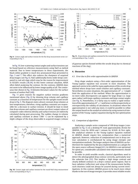
Fig. 11. Drop volume and capillary constant for the round drop measurement series
corresponding to Figs. 5 and 8.
In Fig. 10, low-scattering contact angles and surface tensions can
be found based on reference measurements using NaCl as melted
material. Due to lower temperatures in these experiments, the
black-white-gradient is much less pronounced than presented in
Figs. 5 and 7. This effect also reduces the sharpness of acquired
drop images (see Fig. 6). NaCl additionally forms wider drops compared
to coal ash slags which may be the reason for improvement
in SCA20’s results [38,39]. In this lower contrast situation, ADSA
often failed analysing the contour. On the contrary, LBADSA does
not seem to be influenced by lower image quality at all. The continuous
line shown in Fig. 10 denotes literature values for the surface
tension of molten NaCl [40].
Fig. 11 gives reasons for negative surface tension gradients
mentioned above (Fig. 8) by showing drop volume and capillary
constant as a function of temperature for the upright round sessile
drop in Fig. 5. The diagram states almost constant drop volumes at
low temperatures, therefore, rising capillary constants are responsible
for a decrease in surface tension. It should be kept in mind
that drop volume and capillary constant are direct output values of
computer codes whereas density and surface tension are indirectly
calculated during post-processing. The sudden change in volume
and capillary constant at about 1360 ◦ C can be explained by a
slight collapse of the drop observable in acquired images (release
Fig. 10. Contact angle and surface tension for the round NaCl drop measurement
series corresponding to Fig. 6.
of gaseous species formed within the sessile drop due to chemical
reactions of the slag).
4. Discussion
4.1. Error due to first-order approximation in LBADSA
Drop shape analysis using a first-order approximation of the
Young–Laplace equation was accurate in most situations. The
approach seems to be valid for many applications of the sessile drop
method where drops have small volumes and capillary constants.
Nevertheless in some situations, the approximation cb 2 ≪ 1 might
limit the application of the method. When the approximation is
no more valid, discrepancies can appear for large drops (i.e. large
apex radius) with large capillary constants and large contact angles
(see Fig. 4). Nonetheless, it is fairly easy to realise a rapid estimation
of the approximation cb 2 ≪ 1 and hence verify prospectively or
retrospectively the validity of calculations. In situations where the
approximation is not valid any more, it could be possible to refine
the output based on the analytical solution by using numerical integration
of the Young–Laplace equation during the last optimisation
steps.
4.2. Comparison of algorithms
Analysing a sample series composed of 100 drop images (comparable
to Fig. 5) on a desktop PC took approximately 26 min for
LBADSA, 2 min for ADSA and 1 minute for SCA20. At first sight,
the analytical solution to the Young–Laplace equation realised
in LBADSA should require less computation than a numerical
approach. However, reduction of computational cost in drop contour
calculation is overbalanced by using image energies and
interpolation methods. The longer analysis time of LBADSA can furthermore
be explained by the Java implementation as a plugin for
the open-source software ImageJ [41]. As LBADSA is not optimised
for speed yet, considerable calculation time improvements should
be possible.
In order to yield sensible results, classical algorithms need to
detect the photographed drop contour correctly, particularly near
the substrate line [32]. This implies a high image contrast and
clearly defined contours in a drop’s contact point regions. Due to
heat radiation (reflection) and setup of the measurement facility,
such clearness could not always be assured during current investigations.
In this context, LBADSA proves to be much more robust
thanks to the use of image energies. It provides most reliable results