Computer Tools for Bifurcation Analysis: General Approach with
Computer Tools for Bifurcation Analysis: General Approach with
Computer Tools for Bifurcation Analysis: General Approach with

Create successful ePaper yourself
Turn your PDF publications into a flip-book with our unique Google optimized e-Paper software.
Tutorials and Reviews<br />
International Journal of <strong>Bifurcation</strong> and Chaos, Vol. 9, No. 6 (1999) 983–1008<br />
c○ World Scientific Publishing Company<br />
COMPUTER TOOLS FOR BIFURCATION ANALYSIS:<br />
GENERAL APPROACH WITH APPLICATION TO<br />
DYNAMICAL AND DISTRIBUTED SYSTEMS<br />
LEONID M. PISMEN and BORIS Y. RUBINSTEIN<br />
Department of Chemical Engineering,<br />
Technion — I.I.T., Technion City,<br />
Haifa 32 000, Israel<br />
Received February 2, 1996; Revised December 15, 1998<br />
A general approach of the automated algorithms <strong>for</strong> derivation of amplitude equations <strong>for</strong> dynamical<br />
and distributed systems is presented. A brief description of the Mathematica functions<br />
designed using this approach is given. Application of the functions is illustrated by several<br />
examples dealing <strong>with</strong> dynamical and distributed systems.<br />
1. Introduction . . . . . . . . . . . . . . . . . . . . . . . . . . . . . . . . 984<br />
2. <strong>Bifurcation</strong>s of Dynamical Systems . . . . . . . . . . . . . . . . . . . . . . . 986<br />
2.1. Multiscale Expansion . . . . . . . . . . . . . . . . . . . . . . . . . . 986<br />
2.2. Monotonic <strong>Bifurcation</strong> . . . . . . . . . . . . . . . . . . . . . . . . . . 987<br />
2.2.1 Fold <strong>Bifurcation</strong> . . . . . . . . . . . . . . . . . . . . . . . . . 987<br />
2.2.2 Transcritical <strong>Bifurcation</strong> . . . . . . . . . . . . . . . . . . . . . . 987<br />
2.2.3 Higher-Order <strong>Bifurcation</strong>s . . . . . . . . . . . . . . . . . . . . . 988<br />
2.3. Hopf <strong>Bifurcation</strong> . . . . . . . . . . . . . . . . . . . . . . . . . . . . 988<br />
2.4. Automated Generation of Normal Forms . . . . . . . . . . . . . . . . . . 990<br />
2.5. Computation of Coefficients . . . . . . . . . . . . . . . . . . . . . . . 992<br />
2.5.1 Function CalculateCoefficient . . . . . . . . . . . . . . . . . . . 992<br />
2.5.2 Lorenz Model . . . . . . . . . . . . . . . . . . . . . . . . . . . 992<br />
2.5.3 Brusselator Model . . . . . . . . . . . . . . . . . . . . . . . . . 992<br />
2.5.4 Exothermic Reaction in a Stirred Tank Reactor . . . . . . . . . . . . 993<br />
3. <strong>General</strong> Algorithm <strong>for</strong> Distributed Systems . . . . . . . . . . . . . . . . . . . 995<br />
3.1. Introduction . . . . . . . . . . . . . . . . . . . . . . . . . . . . . . 995<br />
3.2. Linear <strong>Analysis</strong> and Dispersion Relation . . . . . . . . . . . . . . . . . . 996<br />
3.3. Multiscale Expansion . . . . . . . . . . . . . . . . . . . . . . . . . . 996<br />
3.4. Function <strong>Bifurcation</strong>Theory . . . . . . . . . . . . . . . . . . . . . . . 997<br />
4. Amplitude Equations <strong>for</strong> Reaction–Diffusion Problems . . . . . . . . . . . . . . 998<br />
4.1. Long-Scale Instabilities . . . . . . . . . . . . . . . . . . . . . . . . . 998<br />
4.2. Turing <strong>Bifurcation</strong> . . . . . . . . . . . . . . . . . . . . . . . . . . . 999<br />
4.2.1 Hopf <strong>Bifurcation</strong> . . . . . . . . . . . . . . . . . . . . . . . . 1000<br />
983
984 L. M. Pismen & B. Y. Rubinstein<br />
4.3. Brusselator Model . . . . . . . . . . . . . . . . . . . . . . . . . . 1000<br />
4.3.1 Monotonic <strong>Bifurcation</strong> . . . . . . . . . . . . . . . . . . . . . . 1000<br />
4.3.2 Oscillatory <strong>Bifurcation</strong> . . . . . . . . . . . . . . . . . . . . . . 1001<br />
4.4. Two-Level Laser Model . . . . . . . . . . . . . . . . . . . . . . . . 1001<br />
4.4.1 Oscillatory <strong>Bifurcation</strong> . . . . . . . . . . . . . . . . . . . . . . 1001<br />
5. Amplitude Equations <strong>for</strong> Convective Problems . . . . . . . . . . . . . . . . . 1002<br />
5.1. Convective Instabilities . . . . . . . . . . . . . . . . . . . . . . . . 1002<br />
6. Resonant and Degenerate Cases . . . . . . . . . . . . . . . . . . . . . . . 1003<br />
6.1. Three-Wave Resonance in Turing <strong>Bifurcation</strong> . . . . . . . . . . . . . . . 1003<br />
6.1.1 <strong>General</strong> Results . . . . . . . . . . . . . . . . . . . . . . . . . 1003<br />
6.1.2 Calculations <strong>for</strong> Brusselator Model . . . . . . . . . . . . . . . . 1004<br />
6.2. Four-Wave Resonance in Oscillatory Instability . . . . . . . . . . . . . . 1005<br />
6.3. Algebraic Degeneracy — Hopf–Turing <strong>Bifurcation</strong> . . . . . . . . . . . . . 1005<br />
A Linear <strong>Analysis</strong> and Amplitude Equations <strong>for</strong> Lorenz Model . . . . . . . . . . . 1006<br />
B Linear <strong>Analysis</strong> <strong>for</strong> Brusselator Model . . . . . . . . . . . . . . . . . . . . 1007<br />
1. Introduction<br />
Amplitude equations describe behavior of evolutionary<br />
systems in the vicinity of threshold, or critical<br />
values of parameters that mark a point of qualitative<br />
change in behavior, like a transition from<br />
a quiescent state to convection, or from rigid mechanical<br />
equilibrium to vibration, or from a homogeneous<br />
to patterned state of a material medium.<br />
Near the criticality, the behavior of systems of different<br />
physical origin is described by representative<br />
equations belonging to one of the universal<br />
classes that are determined by the character of the<br />
transition.<br />
A common procedure of derivation of amplitude<br />
equations starts from a certain system of evolution<br />
equations symmetric to spatial translations and rotations<br />
and time translations; a necessary condition<br />
is that it does not include explicit dependence on<br />
spatial coordinates and time. This underlying system<br />
may be, in the order of ascending complexity,<br />
a dynamical system (autonomous ODEs), an autonomous<br />
distributed system described by PDEs but<br />
not restricted by boundary conditions, and a distributed<br />
system <strong>with</strong> vertical structure constrained<br />
by boundary conditions along some spatial coordinates<br />
but retaining translational symmetry in other<br />
(unconstrained) directions. A solution that retains<br />
all symmetries of the underlying system is called<br />
a basic state. This state may become unstable to<br />
infinitesimal pertubations in a certain parametric<br />
domain. The instability may be connected <strong>with</strong> the<br />
emergence of new solutions <strong>with</strong> a more complicated<br />
spatiotemporal structure.<br />
In dynamical systems, possible transitions are<br />
bifurcation of multiple stationary states (monotonic<br />
bifurcation) or transition to oscillatory behavior<br />
(Hopf bifurcation). If the phase trajectory of the<br />
dynamical system remains in the vicinity of the basic<br />
state even after the latter becomes unstable,<br />
it can be replaced there by certain reduced equations<br />
called normal <strong>for</strong>ms [Guckenheimer & Holmes,<br />
1983; Hale & Koçak, 1991]. In distributed systems<br />
there are two more possibilities: transition to a stationary<br />
pattern (Turing bifurcation) or to a wave<br />
pattern (Hopf bifurcation at nonzero wavenumber).<br />
Like normal <strong>for</strong>ms of dynamical systems, amplitude<br />
equations describe behavior in the vicinity of the<br />
basic state; they may include, however, also differential<br />
terms describing spatial inhomogeneities on<br />
an extended scale or spatial modulation of a primary<br />
pattern.<br />
There is a number of celebrated “universal”<br />
equations which have been extensively studied in<br />
physical literature. The general structure of these<br />
equations can be often predicted by symmetry considerations.<br />
Some of them were first suggested as<br />
models, others were derived as rational approximations<br />
in a certain physical context, and then discovered<br />
again in apparently unrelated problems. Although<br />
these equations, strictly speaking, may be<br />
valid only in a very limited parametric domain, they<br />
retain a variety of dynamic behavior due to a high
<strong>Computer</strong> <strong>Tools</strong> <strong>for</strong> <strong>Bifurcation</strong> <strong>Analysis</strong> 985<br />
parametric sensitivity in the vicinity of a transition<br />
point. Parametric boundaries between regions<br />
of qualitatively different dynamic behavior can be<br />
drawn as relations between coefficients of amplitude<br />
equations or normal <strong>for</strong>ms. If these coefficients, in<br />
their turn, are expressed through measurable physical<br />
parameters, the boundaries can be mapped upon<br />
the actual parameter space, and then further continued<br />
into a region where universal equations are<br />
no longer valid quantitatively but still faithfully describe<br />
qualitative features of behavior of a complex<br />
nonlinear system.<br />
It is important there<strong>for</strong>e not only to be able<br />
to predict a general <strong>for</strong>m of amplitude equations or<br />
normal <strong>for</strong>ms appropriate to different kinds of bifurcations<br />
but to have at hand reliable tools <strong>for</strong> actual<br />
computation of their coefficients, starting <strong>with</strong><br />
specific underlying evolution equations. The applicable<br />
algorithms, known as center manifold methods<br />
in mathematical literature [Guckenheimer &<br />
Holmes, 1983; Hale & Koçak, 1991], or elimination<br />
of “slaved” variables in physical literature [Haken,<br />
1987], are well established, at least in standard<br />
cases. Actual computations are, however, repetitive<br />
and time-consuming, and have been carried out in<br />
scientific literature on a case-to-case basis. Only<br />
very rarely can they be done manually by anybody<br />
lacking Leverrier’s patience. Application of modern<br />
computer algebra systems — first, REDUCE<br />
and MACSYMA, and later, MAPLE and Mathematica<br />
— is an obvious remedy. It is difficult to<br />
estimate, to what extent they are used nowadays<br />
<strong>for</strong> the study of specific bifurcation problems, as it<br />
is not always explicitly acknowledged in resulting<br />
publications. A case-to-case application is, however,<br />
still arduous and inefficient, compared to the<br />
realization of a general algorithm.<br />
A MACSYMA-based (not fully automated) algorithm<br />
<strong>for</strong> derivation of normal <strong>for</strong>ms of dynamical<br />
systems has been written by Rand and Armbruster<br />
[1987]. Another well-known bifurcation analysis<br />
package AUTO by Doedel, as well as the algorithm<br />
by Guckenheimer et al. [1997] <strong>for</strong> the analysis of<br />
Hopf bifurcation, are restricted to numerical tracking<br />
of solutions of dynamical systems. No general<br />
computer-aided algorithms have been suggested so<br />
far, to the best of the authors’ knowledge, <strong>for</strong> the<br />
analysis of bifurcations in distributed systems.<br />
This tutorial review describes a Mathematicabased<br />
automated algorithm <strong>for</strong> the derivation of<br />
amplitude equations <strong>for</strong> both dynamical and distributed<br />
systems in either symbolic or numerical<br />
<strong>for</strong>m. The algorithm makes use of Mathematica<br />
capabilities as a programming language [Wolfram,<br />
1991, 1996] that allows to define special functions<br />
carrying out complicated tasks in response to simple<br />
and well-defined inputs.<br />
In the course of our work on this algorithm,<br />
we arrived at the conclusion that computations are<br />
most efficient, in terms of CPU time and computer<br />
resourses, when any specific bifurcation problem is<br />
approached as a part of a broader class of problems<br />
leading to an amplitude equation of the same<br />
structure. Accordingly, all computations are carried<br />
out in two stages. The general algorithm based<br />
on multiscale bifurcation expansion is implemented<br />
by the function <strong>Bifurcation</strong>Theory. The input of<br />
this function must be given in a generalized <strong>for</strong>m,<br />
<strong>with</strong>out specifying particular nonlinear functions,<br />
eigenvectors, etc. The inderlying system should be<br />
defined as a single operator equation where various<br />
vectors or arrays are denoted by symbols rather<br />
than being specified explicitly. The output depends<br />
there<strong>for</strong>e only on the type of the bifurcation, applicable<br />
symmetries and the desired order of expansion.<br />
It includes the amplitude equation and unresolved<br />
expressions <strong>for</strong> its coefficients, written in a<br />
generalized symbolic <strong>for</strong>m and containing unimplemented<br />
inverse operators.<br />
The next stage is the actual computation implemented<br />
by the function CalculateCoefficient.<br />
It takes the necessary data <strong>for</strong> a specific system and<br />
uses them in the output of <strong>Bifurcation</strong>Theory to<br />
produce either explicit symbolic expressions <strong>for</strong> coefficients<br />
or their numerical values. Thus, the program<br />
works much in the way as an intelligent mathematician<br />
would: first preparing general <strong>for</strong>mulae<br />
and then working out a specific example. This gives<br />
an order of magnitude acceleration compared to an<br />
earlier version of our algorithm [Pismen et al., 1996]<br />
where amplitude equations containing explicit expressions<br />
<strong>for</strong> coefficients were computed directly <strong>for</strong><br />
specific problems.<br />
The paper is organized as follows. Although<br />
one and the same internal algorithm works <strong>for</strong><br />
dynamic and distributed systems, we start, <strong>for</strong><br />
pedagogical reasons, <strong>with</strong> a detailed treatment<br />
of dynamical systems in Sec. 2. First, the<br />
general algorithm based on multiscale bifurcation<br />
expansion is outlined, and then the function<br />
<strong>Bifurcation</strong>Theory designed to implement this algorithm<br />
is introduced and applied to both monotonic<br />
and Hopf bifurcations. This is followed by<br />
specific examples.
986 L. M. Pismen & B. Y. Rubinstein<br />
Starting from Sec. 3, we repeat the same scheme<br />
<strong>for</strong> distributed systems. The general algorithm is<br />
outlined in Sec. 3 <strong>for</strong> a problem written in the most<br />
general nonlinear operator <strong>for</strong>m. In Sec. 4, the function<br />
<strong>Bifurcation</strong>Theory is applied to reaction–<br />
diffusion problems, followed by specific examples of<br />
computation of coefficients.<br />
In Sec. 5, we consider along the same lines<br />
some problems involving convection that cannot<br />
be reduced to a reaction–diffusion <strong>for</strong>m. Resonant<br />
and algebraically degenerate cases are discussed in<br />
Sec. 6. The primary cause of degeneracy in distributed<br />
systems <strong>with</strong> two unrestrained direction<br />
is rotational symmetry that makes excitation of<br />
stationary inhomogeneities or waves <strong>with</strong> different<br />
directions of the wavenumber vector. Strong resonances<br />
may involve in such systems three wave<strong>for</strong>ms<br />
in the case of a monotonic (Turing), and four<br />
wave<strong>for</strong>ms in the case of a wave (Hopf) bifurcation.<br />
We shall also give an example of a parametric<br />
(“accidental”) degeneracy involving mixed Hopf<br />
and Turing modes. The algorithm is applicable only<br />
when the degeneracy is algebraic but not geometric.<br />
The latter case requires essential modification of the<br />
multiscale expansion procedure, and is outside the<br />
scope of this communication.<br />
2. <strong>Bifurcation</strong>s of Dynamical Systems<br />
2.1. Multiscale expansion<br />
The standard general algorithm <strong>for</strong> derivation of<br />
amplitude equations (normal <strong>for</strong>ms) is based on<br />
multiscale expansion of an underlying dynamical<br />
system in the vicinity of a bifurcation point. Consider<br />
a set of first-order ordinary differential equations<br />
in R n :<br />
du/dt = f(u, R) , (1)<br />
where f(u; R) is a real-valued n-dimensional<br />
vector-function of an n-dimensional array of dynamic<br />
variables u, that is also dependent on an<br />
m-dimensional array of parameters R. We expand<br />
both variables and parameters in powers of<br />
a dummy small parameter ε:<br />
u = u 0 + εu 1 + ε 2 u 2 + ··· ,<br />
R=R 0 +εR 1 +ε 2 R 2 +···<br />
(2)<br />
Next, we introduce a hierarchy of time scales t k<br />
rescaled by the factor ε k , thereby replacing the function<br />
u(t) by a function of an array of rescaled time<br />
variables. Accordingly, the time derivative is expanded<br />
in a series of partial derivatives ∂ k ≡ ∂/∂t k :<br />
d<br />
dt = ∂ 0 + ε∂ 1 + ε 2 ∂ 2 + ··· . (3)<br />
Let u = u 0 (R 0 ) be an equilibrium (a fixed<br />
point) of the dynamical system (1), i.e. a zero of<br />
the vector-function f(u; R) atapointR=R 0 in<br />
the parametric space. The function f(u; R) canbe<br />
expanded in the vicinity of u 0 , R 0 in Taylor series<br />
in both variables and parameters:<br />
f(u; R) =f u (u−u 0 )+ 1 2 f uu(u − u 0 ) 2<br />
+ 1 6 f uuu(u − u 0 ) 3 + ···+f R (R−R 0 )<br />
+ f uR (u − u 0 )(R − R 0 )<br />
+ 1 2 f uuR(u − u 0 ) 2 (R − R 0 )+··· .<br />
(4)<br />
The derivatives <strong>with</strong> respect to both variables and<br />
parameters f u = ∂f/∂u, f uu = ∂ 2 f/∂u 2 , f R =<br />
∂f/∂R, f uR = ∂ 2 f/∂u∂R, etc. are evaluated at<br />
u = u 0 , R = R 0 .<br />
Using Eqs. (2)–(4) in Eq. (1) yields in the firstorder<br />
∂ 0 u 1 = f u u 1 + f R R 1 . (5)<br />
The homogeneous linear equation<br />
Lu 1 ≡ (f u − ∂/∂t 0 )u 1 =0 (6)<br />
obtained by setting in Eq. (5) R 1 = 0 governs<br />
the stability of the stationary state u = u 0 to infinitesimal<br />
perturbations. The state is stable if all<br />
eigenvalues of the Jacobi matrix f u have negative<br />
real parts. This can be checked <strong>with</strong> the help of<br />
the standard Mathematica function Eigenvalues.<br />
Computation of all eigenvalues is, however, superfluous,<br />
since stability of a fixed point is determined<br />
by the location in the complex plane of a leading<br />
eigenvalue, i.e. <strong>with</strong> the largest real part. Generically,<br />
the real part of the leading eigenvalue vanishes<br />
on a codimension one subspace of the parametric<br />
space called a bifurcation manifold. The two types<br />
of codimension one bifurcations that can be located<br />
by local (linear) analysis are a monotonic bifurcation<br />
where a real leading eigenvalue vanishes, and<br />
a Hopf bifurcation where a leading pair of complex<br />
conjugate eigenvalues is purely imaginary. Additional<br />
conditions may define bifurcation manifolds<br />
of higher codimension.
<strong>Computer</strong> <strong>Tools</strong> <strong>for</strong> <strong>Bifurcation</strong> <strong>Analysis</strong> 987<br />
2.2. Monotonic bifurcation<br />
2.2.1. Fold bifurcation<br />
A monotonic bifurcation is also a bifurcation of<br />
equilibria of the dynamical system (1). Setting u 1<br />
= const, i.e. ∂ 0 u 1 = 0, allows to find a shift of<br />
the stationary solution due to small variations of<br />
parameters<br />
u 1 = −fu −1 f R R 1 . (7)<br />
The n × m array fu<br />
−1f<br />
R is recognized as the parametric<br />
sensitivity matrix. Continuous dependence<br />
on parameters can be used to construct a branch of<br />
equilibria which terminates at a bifurcation point<br />
R 0 .<br />
On a monotonic bifurcation manifold, the matrix<br />
f u has no inverse. This means that one can<br />
neither construct a stationary solution at values of<br />
parameters close to this point, nor characterize the<br />
stability of the equilibrium in the linear approximation.<br />
The dynamics in the vicinity of the bifurcation<br />
manifold is governed by a nonlinear amplitude<br />
equation to be obtained in higher orders of the<br />
expansion.<br />
Generically, the zero eigenvalue is nondegenerate.<br />
Let U be the corresponding eigenvector satisfying<br />
f u U =0. Then<br />
u 1 =a(t 1 ,t 2 ,...)U (8)<br />
is the solution of Eq. (6) that remains stationary<br />
on the fast time scale t 0 . The amplitude a is so<br />
far indeterminate, and can depend on slower time<br />
scales.<br />
The inhomogeneous equation (5) has solutions<br />
constant on the rapid time scale, provided its inhomogeneity<br />
does not project on the eigenvector U.<br />
This condition is<br />
κ 1 ≡ U † f R R 1 =0, (9)<br />
where U † is the eigenvector of the transposed matrix<br />
f u † = Transpose[f u ] satisfying f u † U † =0;weassume<br />
that the eigenvector is normalized: U † U =1.<br />
Equation (9) defines the tangent hyperplane to the<br />
bifurcation manifold at the point R = R 0 .<br />
Be<strong>for</strong>e writing up the second-order equation,<br />
we require that the second-order deviation u 2 remain<br />
constant on the rapid time scale (otherwise it<br />
might outgrow u 1 at long times). The dependence<br />
upon slower time scales must be expressed exclusively<br />
through the time dependence of the amplitude<br />
a. Using Eq. (8), we write the second-order<br />
equation as<br />
f u u 2 = ∂ 1 aU − f R R 2 − af uR UR 1 − 1 2 a2 f uu UU .<br />
(10)<br />
The solvability condition of this equation is<br />
∂ 1 a = κ 2 + λ 1 a + µ 0 a 2 . (11)<br />
The parameters of Eq. (11) are<br />
κ 2 = U † f R R 2 + 1 2 U† f RR R 1 R 1 ,<br />
λ 1 = U † f uR UR 1 ,<br />
µ 0 = 1 2 U† f uu UU .<br />
(12)<br />
The indices correspond to the scaling of respective<br />
parametric deviations from the bifurcation point.<br />
In a generic case, one can consider only parametric<br />
deviations transverse to the bifurcation manifold,<br />
and set R 1 = 0 to satisfy Eq. (9); then λ 1 =0,and<br />
generic equation <strong>for</strong> slow dynamics near the bifurcation<br />
manifold becomes<br />
∂ 1 a = κ 2 + µ 0 a 2 . (13)<br />
This equation can be also obtained by shifting the<br />
amplitude in Eq. (11). On the one side of the bifurcation<br />
manifold, where κ 2 has the sign opposite<br />
to that of µ 0 , there are two stationary states<br />
a = ± √ −κ 2 /µ 0 . When viewed as a solution of<br />
Eq. (13), one of them is stable, and the other, unstable.<br />
The stable solution corresponds to a stable<br />
equilibrium of the original system Eq. (1), provided<br />
the rest of eigenvalues of the matrix f u have negative<br />
real parts. On the other side of the bifurcation<br />
manifold, where the signs κ 2 and µ 0 are the same,<br />
there are no stationary states. The trajectory of<br />
the dynamical system is deflected then to another<br />
attractor, far removed from u 0 . Thus, the system<br />
undergoes a first-order phase transition when the<br />
bifurcation manifold is crossed. If the value of some<br />
dynamic variable or other characteristic of the solution<br />
is drawn as a function of parameters, the bifuration<br />
locus can be seen as the projection of a fold of<br />
the solution manifold on the parametric plane; accordingly,<br />
the generic monotonic bifurcation is also<br />
called a fold bifurcation.<br />
2.2.2. Transcritical bifurcation<br />
It may happen that the matrix f R as well the tensor<br />
f RR vanish identically. This would be the case when<br />
u 0 is a “trivial” solution that remains constant at
988 L. M. Pismen & B. Y. Rubinstein<br />
all values of parameters. Then Eq. (9) is satisfied<br />
identically, and Eq. (11) reduces to<br />
∂ 1 a = λ 1 a + µ 0 a 2 . (14)<br />
This equation has two solutions, a =0anda=<br />
−λ 1 /µ 0 , on both sides of the bifurcation manifold,<br />
but the two solutions interchange stability when<br />
this manifold is crossed. This bifurcation is called<br />
transcritical.<br />
2.2.3. Higher-order bifurcations<br />
If µ 0 = 0, the expansion should be continued to<br />
the next order. The coefficient µ 0 may vanish identically<br />
due to the symmetry of the original problem<br />
to inversion of u. Otherwise, it can be equal<br />
to zero at certain values of the parameters of the<br />
problem. <strong>General</strong>ly, the two conditions, Det[f u ]=0<br />
and µ 0 = 0 are satisfied simultaneously on a codimension<br />
two manifold in the parametric space that<br />
corresponds to a cusp singularity.<br />
In order to continue the expansion, we restrict<br />
parametric deviations in such a way that the dependence<br />
on t 1 be suppressed. Deviations transverse<br />
to the bifurcation manifold have to be restricted<br />
by the condition κ 2 = 0, which is stronger than<br />
Eq. (9). First-order parametric deviations R 1 parallel<br />
to the bifurcation manifold, which are still allowed<br />
by Eq. (9), should be now restricted by the<br />
condition λ 1 = 0. If the array R contains two parameters<br />
only, the conditions λ 1 =0andκ 1 =0imply,<br />
in a nondegenerate case, that first-order parametric<br />
deviations should vanish identically. When<br />
more parameters are available, parametric deviations<br />
satisfying both these conditions are superfluous,<br />
since they correspond just to gliding into a<br />
closer vicinity of another point on the cusp bifurcation<br />
manifold in a higher-dimensional parametric<br />
space. Further on, we shall set there<strong>for</strong>e R 1 to zero<br />
identically.<br />
The dynamics unfolding on a still slower time<br />
scale t 2 should be determined from the third-order<br />
equation<br />
f u u 3 = ∂ 2 aU − f R R 3 − af uR UR 2<br />
− af uu Uu 2 − 1 6 a3 f uuu UUU . (15)<br />
The second-order function u 2 has to be found by<br />
solving Eq. (10), now reduced to the <strong>for</strong>m<br />
f u u 2 = −f R R 2 − 1 2 a2 f uu UU . (16)<br />
Only the solution of the inhomogeneous equation,<br />
which does not project on the eigenvector U, isrelevant.<br />
It can be expressed as<br />
u 2 = U (2)<br />
2 + a 2 U (0)<br />
2 . (17)<br />
The solvability condition of Eq. (15) is obtained<br />
then in the <strong>for</strong>m<br />
where<br />
∂ 2 a = κ 3 + λ 2 a + ν 0 a 3 , (18)<br />
κ 3 = U † f R R 3 ,<br />
λ 2 = U † f uR UR 2 + U † f uu UU (2)<br />
2 ,<br />
ν 0 = 1 6 U† f uuu UUU + U † f uu UU (0)<br />
2 . (19)<br />
Equation (18) presents a parametric unfolding<br />
of dynamics in the vicinity of a cusp bifurcation.<br />
Three equilibria — two stable and one unstable —<br />
exist in the cusped region<br />
λ 2 > 0 , |κ 3 | < 2λ3/2<br />
3 3/2 . (20)<br />
ν1/2 Outside this region, there is a unique stable equilibrium.<br />
A second-order phase transition occurs when<br />
the parameters change in such a way that λ 2 crosses<br />
zero. Other transitions occuring in the vicinity of<br />
the cusp bifurcation are weakly first-order.<br />
The condition ν 0 = 0 defines a singular bifurcation<br />
manifold of codimension three. Again, it is<br />
possible to fix parametric deviations to suppress the<br />
dynamics on the scale t 2 , and obtain in the next<br />
order a quartic equation that represents the unfolding<br />
of the butterfly singularity. The procedure can<br />
be continued further if a sufficient number of free<br />
parameters is available. The unfolding of a codimension<br />
q singularity is presented by a polynomial<br />
of order q +1:<br />
q−1<br />
∑<br />
∂ q a= σ q−p+1 a p + σ 0 a q+1 , (21)<br />
p=0<br />
where the parameters σ k depend on parametric deviations<br />
proportional to ε k .<br />
2.3. Hopf bifurcation<br />
At the Hopf bifurcation point the parametric dependence<br />
of the stationary solution u = u 0 (R) remains<br />
smooth; a linear correction can be obtained
<strong>Computer</strong> <strong>Tools</strong> <strong>for</strong> <strong>Bifurcation</strong> <strong>Analysis</strong> 989<br />
from the stationary equation (7), and higher corrections<br />
from higher orders of the regular expansion<br />
(4). In order to simplify derivations, we shall eliminate<br />
this trivial parametric dependence by trans<strong>for</strong>mingtoanewvariableû=u−u<br />
0 (R). The<br />
resulting dynamic system, dû/dt = ˆf(û, R) hasthe<br />
same <strong>for</strong>m as (1) but contains a modified vectorfunction<br />
ˆf(û, R) =f(û+u 0 ,R). Since, by definition,<br />
u 0 satisfies f(u 0 , R) =0,û= 0 is a zero of<br />
ˆf(û, R). Now we can drop the hats over the symbols<br />
and revert to the original <strong>for</strong>m (1) while keeping in<br />
mind that u = 0 is a stationary solution <strong>for</strong> all R<br />
and, consequently, all derivatives f R , f RR ,etc.computed<br />
at u = 0 vanish.<br />
At a Hopf bifurcation point the Jacobi matrix<br />
f u has a pair of imaginary eigenvalues λ = ±iω 0 .<br />
The first-order Eq. (6) has a nontrivial oscillatory<br />
solution<br />
u 1 = a(t 1 ,t 2 ,...)Φ(t 0 )+c.c. ;<br />
Φ(t 0 )=e iω 0t 0<br />
U<br />
(22)<br />
<strong>with</strong> an arbitrary complex amplitude a(t 1 ,t 2 ,...)<br />
dependent on slower time scales t k ,k>0; U is the<br />
eigenvector of f u <strong>with</strong> the eigenvalue iω 0 :<br />
f u U = iω 0 U . (23)<br />
The function Φ(t 0 ) and its complex conjugate<br />
Φ ∗ (t 0 ) are two eigenfunctions of the linear operator<br />
L, Eq. (6), <strong>with</strong> zero eigenvalue. The operator<br />
L acts here in the space of 2π/ω 0 -periodic complexvalued<br />
vector-functions <strong>with</strong> the scalar product defined<br />
as<br />
〈u, v〉 = ω ∫ 2π/ω0<br />
0<br />
u ∗ (t) · v(t)dt . (24)<br />
2π 0<br />
The eigenfunctions of the adjoint operator L † =<br />
f u † + ∂/∂t 0 are<br />
Φ † (t 0 )=e −iω 0t 0<br />
U †<br />
and its complex conjugate; U † is the eigenvector of<br />
f u † <strong>with</strong> the eigenvalue iω 0 .<br />
The second-order equation can be written in<br />
the <strong>for</strong>m<br />
Lu 2 = ∂ 1 u 1 − 1 2 f uuu 1 u 1 − f uR u 1 R 1 . (25)<br />
zero and double frequency stemming from the<br />
quadratic term 1/2f uu u 1 u 1 . The scalar products<br />
of the latter terms <strong>with</strong> the eigenfunctions<br />
Φ † (t 0 ), Φ †∗ (t 0 ) vanish, and the solvability condition<br />
of Eq. (25) is obtained in the <strong>for</strong>m:<br />
∂ 1 a = λ 1 a, (26)<br />
where λ 1 is given by Eq. (12) (note that this parameter<br />
is now complex).<br />
Equation (26) has a nontrivial stationary solution<br />
only if the real part of λ 1 vanishes. This condition<br />
defines a hyperplane in the parametric space<br />
tangential to the Hopf bifurcation manifold. The<br />
imaginary part of λ 1 gives a frequency shift along<br />
the bifurcation manifold. In order to eliminate the<br />
tangential shift, we set as be<strong>for</strong>e R 1 =0. Then<br />
Eq. (26) reduces to ∂ 1 a = 0, so that the amplitude<br />
may evolve only on a still slower scale t 2 .The<br />
second-order function u 2 has to be found by solving<br />
Eq. (25), now reduced to the <strong>for</strong>m<br />
Lu 2 = − 1 2 (a2 e 2iω 0t 0<br />
f uu UU + |a| 2 f uu UU ∗ + c.c) .<br />
(27)<br />
The solution of this equation is<br />
u 2 = − 1 2 [|a|2 f u −1 f uu UU ∗<br />
+ a 2 e 2iω 0t 0<br />
(f u − 2iω 0 ) −1 f uu UU + c.c.] . (28)<br />
In the third-order,<br />
Lu 3 = ∂ 2 u 1 − f uR u 1 R 2<br />
− f uu u 1 u 2 − 1 6 f uuuu 1 u 1 u 1 . (29)<br />
The amplitude equation is obtained as the solvability<br />
condition of this equation. Only the part of the<br />
inhomogeinity containing the principal harmonic<br />
contributes to the solvability condition, which takes<br />
the <strong>for</strong>m<br />
∂ 2 a = λ 2 a + ν 0 |a| 2 a, (30)<br />
where λ 2 ,ν 0 are defined as<br />
λ 2 = U † f uR UR 2 ,<br />
ν 0 = 1 2 U† f uuu UUU ∗ − U † f uu U(f u −1 f uu UU ∗ )<br />
The inhomogeinity of this equation contains both<br />
the principal harmonic, e iω 0t 0<br />
, contributed by the<br />
linear terms ∂ 1 u 1 and f uR u 1 R 1 , and terms <strong>with</strong><br />
− 1 2 U† f uu U ∗ ((f u − 2iω 0 ) −1 f uu UU) .<br />
(31)
990 L. M. Pismen & B. Y. Rubinstein<br />
The expansion has to be continued to higher orders,<br />
after readjusting the scaling of parametric deviations,<br />
if the real part of ν 0 vanishes.<br />
2.4. Automated generation<br />
of normal <strong>for</strong>ms<br />
The procedure of derivation of a sequence of amplitude<br />
equations described in the preceding section is<br />
implemented by the function <strong>Bifurcation</strong>Theory.<br />
<strong>Bifurcation</strong>Theory[operatoreqn, u, R, t, {U,<br />
U † }, amp, coef, eps, order, freq, options] derives<br />
a set of amplitude equations <strong>for</strong> a dynamical system<br />
of ordinary differential equations written in an operator<br />
<strong>for</strong>m.<br />
<strong>Bifurcation</strong>Theory has the following arguments:<br />
• operatoreqn denotes an operator equation describing<br />
the problem;<br />
• u denotes a array of variables;<br />
• R denotes a array of bifurcation parameters;<br />
• t denotes a time variable;<br />
• U and U † stand <strong>for</strong> the normal mode eigenvectors;<br />
• amp is an amplitude of the normal mode appearing<br />
in the linear solution;<br />
• coef denotes the name of coefficients of the resulting<br />
amplitude equations;<br />
• eps denotes the small parameter of the problem<br />
(ε);<br />
• order is the highest order of the expansion; if it<br />
is higher than the codimension of the bifurcation<br />
manifold, corrections to the principal (lowest order)<br />
amplitude equation are produced;<br />
• freq denotes the frequency of the arising limit<br />
cycle (<strong>for</strong> monotonic bifurcations it can be<br />
dropped).<br />
The differentiation operator ∂/∂t used in the<br />
operator equation operatoreqn is represented by<br />
the symbols Nabla[t]. Action of this operator on<br />
functional expressions is denoted by the symbol ∗∗<br />
— alias to NonCommutativeMultiply.<br />
The function <strong>Bifurcation</strong>Theory admits the<br />
option ScalarProduct specifying a pure function<br />
<strong>for</strong> scalar product used in solvability condition. The<br />
default value is ScalarProduct -> Dot.<br />
As it is discussed in the preceeding section the<br />
function automatically shifts the basic solution in<br />
the process of derivation of the normal <strong>for</strong>ms <strong>for</strong><br />
Hopf bifurcation. As <strong>for</strong> monotonic bifurcations<br />
there is no shift <strong>with</strong> only one exception. In case of<br />
transcritical monotonic bifurcation, where the basic<br />
state solution remains constant at all values of<br />
parameter, the shift of the solution is admissible.<br />
This case needs an application of another option<br />
Transcritical -> True which <strong>for</strong>ces the function<br />
to make a shift in monotonic case. The default value<br />
of this option is Transcritical -> False.<br />
As an example of usage of the function<br />
<strong>Bifurcation</strong>Theory, we consider the Hopf bifurcation.<br />
Un<strong>for</strong>tunately, the version 2.2.2 of Mathematica<br />
used in development of the package has no<br />
perfect typesetting abilities of the version 3.0. As a<br />
result the output of the function is very lengthy and<br />
is difficult to understand <strong>for</strong> inexperienced users.<br />
We present the Mathematica output only once and<br />
further we will use the standard textbook notation.<br />
The original dynamical problem in the standard<br />
notation has a <strong>for</strong>m:<br />
u t = f(u, R) . (32)<br />
Hence the first argument operatoreqn will take a<br />
<strong>for</strong>m: f[u, R] − Nabla[t]**u == 0 and the function<br />
<strong>Bifurcation</strong>Theory is used as follows:<br />
dynoscbif = <strong>Bifurcation</strong>Theory[<br />
f[u, R] − Nabla[t]**u == 0, u, R, t, {U,<br />
Ut}, a, c, eps, 2, w].<br />
The result produced by the function can be presented<br />
as a set of two amplitude equations describing<br />
the slow dynamics of the amplitude a at the<br />
time scales t i = ε i t 0 , (i =1,2) [cf. Eqs. (26) and<br />
(30)]:<br />
{a (1,0) [t[1], t[2]] == a[t[1], t[2]] c[2,<br />
2][R[1]] / c[2, 1],<br />
a (0,1) [t[1], t[2]] ==<br />
a[t[1], t[2]] 2 Conjugate[a[t[1], t[2]]]<br />
c[3, 2] / c[3, 1] +<br />
a[t[1], t[2]] c[3, 3][R[1], R[2]] / c[3,<br />
1]},<br />
or in the usual notation:<br />
∂ 1 a = c 2, 2(R 1 )<br />
a,<br />
c 2, 1<br />
∂ 2 a= c 3,2<br />
c 3,1<br />
|a| 2 a+ c 3,3(R 1 , R 2 )<br />
c 3,1<br />
a. (33)<br />
The coefficients c ij of the amplitude equations are<br />
generated separately and, hence, can be calculated<br />
and simplified separately. The coefficients c 2, 1 =<br />
c 3, 1 = UU † determine the normalization of the<br />
eigenvectors.
<strong>Computer</strong> <strong>Tools</strong> <strong>for</strong> <strong>Bifurcation</strong> <strong>Analysis</strong> 991<br />
The coefficient in Eq. (26) λ 1 = c 2, 2 (R 1 )/c 2, 1 .<br />
Formulae <strong>for</strong> calculation of coefficients c are given<br />
by the set of the replacement rules:<br />
{c[2, 1] -> Ut . U,<br />
c[2, 2][R[1]] -> Ut . f (1,1) [u, R] . U .<br />
R[1]}.<br />
The second equation is a well-known Landau equation,<br />
and the coefficient at the nonlinear term ν 0 =<br />
c 3, 2 /c 3, 1 is called the Landau coefficient. The sign<br />
of this coefficient determines the type of the bifurcation<br />
— the subcritical one <strong>with</strong> unstable limit cycle<br />
coefficient arises if the real part of the coefficient is<br />
positive, and the supercritical otherwise. The unnormalized<br />
Landau coefficient c 3,2 is produced by<br />
the function in the following <strong>for</strong>m:<br />
c[3, 2] -> -Ut . f (2,0) [u, R] . U .<br />
LinearSolve[f (1,0) [u, R], f (2,0) [u, R] .<br />
DiracConjugate[U] . U] -<br />
Ut . f (2,0) [u, R] . DiracConjugate[U] .<br />
LinearSolve[-2 I w IdentityTensor[2] +<br />
f (1,0) [u, R],<br />
f (2,0) [u, R] . U . U] / 2 +<br />
Ut . f (3,0) [u, R] . DiracConjugate[U] . U .<br />
U / 2,<br />
and can be written in the standard notation as:<br />
c 3, 2 = −U † f uu UR(f u )f uu UŨ<br />
− U † f uu ŨR(−2iwI + f u )f uu UU/2<br />
− U † f uuu UUŨ/2 , (34)<br />
where I denotes the identity matrix, which<br />
corresponds to the IdentityTensor[2] (tensor<br />
of the rank 2) generated by the function<br />
<strong>Bifurcation</strong>Theory. The R(m) denotes the resolvent<br />
matrix of the matrix m — if the matrix is<br />
regular, resolvent coincides <strong>with</strong> the inverse matrix,<br />
otherwise, resovent is constructed using the spectrum<br />
of the original matrix m. A special function<br />
Resolvent[matrix] is designed <strong>for</strong> the construction<br />
of the resolvent of a singular matrix.<br />
Finally the linear term coefficient in the Landau<br />
equation depends on parametric deviations of<br />
the first- and second-order:<br />
c 3, 3 (R 1 , R 2 )<br />
=(U † R(−iwI+f u )f uR UR 1 )(U † f uR UR 1 )/(U † U)<br />
+ U † f uR UR 2 −U † f uR R(−iwI+f u )f uR UR 1 R 1<br />
+ U † f uRR UR 1 R 1 /2 . (35)<br />
It can be easily seen that the condition R 1 = 0<br />
reduces the above general expression to linear coefficient<br />
λ 2 in (31) depending on R 2 only.<br />
The case of a monotonic bifurcation is more<br />
complicated, the resulting <strong>for</strong>mulae are more cumbersome,<br />
and we present the results of the Mathematica<br />
calculations in the standard notation. It<br />
must be noted that it has been indicated in the<br />
previous section that the first-order parametric deviation<br />
R 1 is automatically set to zero.<br />
The set of two amplitude equations describing<br />
the slow dynamics of the amplitude a now takes a<br />
<strong>for</strong>m:<br />
∂ 1 a = c 2, 2<br />
c 2, 1<br />
a 2 + c 2, 3(R 2 )<br />
c 2, 1<br />
,<br />
∂ 2 a = c 3, 2<br />
c 3,, 1<br />
a 3 + c 3, 3(R 2 )<br />
c 3, 1<br />
a + c 3, 4(R 3 )<br />
c 3, 1<br />
.<br />
(36)<br />
Now the nontrivial amplitude equation appears<br />
already at the first time scale t 1 . It contains<br />
quadratic in amplitude term <strong>with</strong> unnormalized coefficient<br />
given by:<br />
c 2, 2 = U † f uu UU/2 , (37)<br />
and corresponds to µ 0 in (12); the coefficient c 2, 3<br />
coincides <strong>with</strong> κ 2 in (12).<br />
The equation at the slower time scale gives corrections<br />
to the principal equation. Its Landau coefficient<br />
can be cast as follows:<br />
c 3, 2 =(U † R(f u )f uu UU)(U † f uu UU)/(2U † U)<br />
− U † f uu UR(f u )f uu UU/2<br />
+ U † f uuu UUU/6 . (38)<br />
The linear term coefficient is given as:<br />
c 3, 3 (R 2 )<br />
= U † f uR UR 2<br />
+(U † R(f u )f uu UU)(U † f uR UR 2 )/(U † U)<br />
− U † f uu UR(f u )f R R 2 .<br />
(39)<br />
Finally the free term in the equation coincides <strong>with</strong><br />
κ 3 in (19).
992 L. M. Pismen & B. Y. Rubinstein<br />
2.5. Computation of coefficients<br />
2.5.1. Function CalculateCoefficient<br />
In order to per<strong>for</strong>m the calculation of the coefficient<br />
of the amplitude equations describing slow<br />
dynamics in the vicinity of a bifurcation point of<br />
a particular problem it is needed to specify values<br />
of all elements in the output of the function<br />
<strong>Bifurcation</strong>Theory, substitute them into the <strong>for</strong>mulae<br />
and carry out required simplifications. The<br />
last two steps of this procedure is per<strong>for</strong>med automatically<br />
by the function CalculateCoefficient.<br />
CalculateCoefficient[coefrule, urule,<br />
Rrule, freqrule, funcrules, eigenrules,<br />
addrules] per<strong>for</strong>ms calculation of the rule <strong>for</strong> the<br />
coefficient of the amplitude equations provided by<br />
the function <strong>Bifurcation</strong>Theory using the rules<br />
specifying the required data.<br />
CalculateCoefficient has the following arguments:<br />
• coefrule denotes a rule <strong>for</strong> the coefficient of the<br />
amplitude equations produced by the function<br />
<strong>Bifurcation</strong>Theory;<br />
• urule specifies the names of the state vector components<br />
<strong>with</strong> their critical values at the bifurcation<br />
point;<br />
• Rrule specifies the names of the bifurcation parameter<br />
vector components <strong>with</strong> their critical values<br />
at the bifurcation point;<br />
• freqrule specifies the values, wavenumber and<br />
frequency at the bifurcation point;<br />
• funcrules denotes an array of rules specifying<br />
all functional and constant objects (array, matrices,<br />
tensors, etc.) appearing in the output of the<br />
function <strong>Bifurcation</strong>Theory;<br />
• eigenrules denotes an array of rules specifying<br />
values of the eigenvectors of the problem;<br />
• addrules denotes an array of additional rules<br />
needed <strong>for</strong> calculations (<strong>for</strong> example, restrictions<br />
on the parametric deviations); this argument can<br />
be dropped.<br />
The function CalculateCoefficient has the<br />
only option ComplexTheory specifying the names<br />
of the state vector components assumed to be<br />
complex-valued. The default value of the option<br />
is ComplexTheory -> None. Example of the usage<br />
in presented in Appendix A.<br />
2.5.2. Lorenz model<br />
The well-known Lorenz system [Lorenz, 1963], that<br />
has been originally suggested as a qualitative model<br />
of cellular convection, exhibits rich dynamic behavior<br />
including periodic and chaotic motion. It also<br />
possesses a monotonic bifurcation that corresponds<br />
to a primary transition from the quiescent state to<br />
convection. In usual notation, the Lorenz system is<br />
written as<br />
dx/dt = −σ(x − y) ,<br />
dy/dt = x(R − z) − y,<br />
dz/dt = −bz + xy .<br />
The linear analysis made <strong>with</strong> Mathematica<br />
which is presented in the Appendix A locates the<br />
bifurcation point at x = y = z =0andR=1;<br />
the eigenvectors are U = {1, 1, 0} and U † =<br />
{1/σ, 1, 0}. Calculations of the coefficients per<strong>for</strong>med<br />
in Appendix A shows that the lowest-order<br />
equation is trivial – ∂ 1 a =0.The Landau equation<br />
has the <strong>for</strong>m:<br />
∂ 2 a =<br />
σ<br />
1+σ (−a3 /b + aR 2 ) .<br />
The result proves that the bifurcation is always<br />
supercritical at physical (positive) values of the<br />
parameters.<br />
2.5.3. Brusselator model<br />
The next example is a well-known Brusselator<br />
model of chemical oscillations [Nicolis & Prigogine,<br />
1977]:<br />
dz/dt = a − (1 + b)z + uz 2 ,<br />
du/dt = bz − uz 2 .<br />
The real variables u, z denote concentrations of the<br />
“activator” and “inhibitor” species. The unique<br />
stationary solution z = a, u = b/a bifurcates into<br />
the limit cycle at b =1+a 2 . Calculations can be<br />
made only after elimination of the parametric dependence<br />
of the basic solution made by the shifting<br />
of the basic solution to zero. The shifted system<br />
has the following <strong>for</strong>m:<br />
dz/dt = a 2 u − z + bz +2auz + bz 2 /a + uz 2 ,<br />
du/dt = −a 2 u − bz − 2auz − bz 2 /a − uz 2 .<br />
The linear analysis of the problem is presented in<br />
Appendix B. The eigenvectors at the Hopf bifurcation<br />
point are U = {a/(i − a), 1} and U † =<br />
{(i + a)/a, 1}.
<strong>Computer</strong> <strong>Tools</strong> <strong>for</strong> <strong>Bifurcation</strong> <strong>Analysis</strong> 993<br />
The calculation produces the following results<br />
<strong>for</strong> the coefficients in the first equation from (33):<br />
c 2, 1 = 2<br />
1+ia ;<br />
Setting b 1<br />
order:<br />
c 2, 2 (R 1 )= b 1<br />
1+ia . (40)<br />
= 0 one can proceed to the next<br />
c 3, 1 = 2<br />
1+ia ;<br />
c 3, 2 = 4 − 6ia − 7a2 − 3ia 3 +4a 4<br />
3ia(1 + a 2 )(1 + ia)<br />
c 3, 3 (R 1 , R 2 )= b 2<br />
1+ia . (41)<br />
The Landau coefficient at the nonlinear term<br />
finally takes a <strong>for</strong>m<br />
4 − 6ia − 7a 2 − 3ia 3 +4a 4<br />
6ia(1 + a 2 ;<br />
)<br />
it is easy to see that its real part simplifies to<br />
−(1 + 1/2a 2 )/(1 + a 2 ), and is negative definite,<br />
hence, the bifurcation is always supercritical.<br />
2.5.4. Exothermic reaction in<br />
a stirred tank reactor<br />
The following example involves somewhat heavier<br />
computations, and necessitates the use of implicit<br />
functions. Consider a dynamical system describing<br />
an exotermic reaction in a continuous stirred tank<br />
reactor [Uppal et al., 1974; Pismen, 1986]:<br />
dx/dt =(1−x)e y −mx ,<br />
(42)<br />
gdy/dt=h(1 − x)e y − my .<br />
The variables x, y denote the conversion and dimensionless<br />
temperature, respectively; h is the exothermicity<br />
parameter, m is the dimensionless flow rate,<br />
and g is the thermal capacitance factor that equals<br />
to unity in an adiabatic reactor and decreases <strong>with</strong><br />
intensified cooling. This model exhibits both monotonic<br />
and Hopf bifurcations. Equilibria of Eq. (42)<br />
do not depend on the parameter g, so conditions of<br />
a monotonic bifurcation can depend on two independent<br />
parameters m, h only; the maximal codimension<br />
is two (a cusp point).<br />
Monotonic bifurcation. Consider first a bifurcation<br />
manifold of codimension one (a fold line)<br />
;<br />
<strong>for</strong> a simplified model <strong>with</strong> g = 1. We localize<br />
this bifurcation as be<strong>for</strong>e — the bifurcation locus<br />
parametrized by the stationary value y s of the variable<br />
y can be found <strong>with</strong> the help of the standard<br />
Mathematica function Solve. This parametrization<br />
is advantageous, since if one of the actual parameters<br />
h or m was used, either two or no solutions<br />
were obtained in different parametric domains, and<br />
the <strong>for</strong>m of the solution was more complicated. The<br />
manifold is given as:<br />
x =1− 1 y s<br />
, m = eys<br />
y s −1 , h = y2 s<br />
y s −1 .<br />
The admissible values of y s are restricted by the<br />
condition y s > 1. The eigenvectors of the problem<br />
can be written as U = {(−1 +y s )/ys 2 , 1} and<br />
U † = {−y s , 1}. The calculation process is similar<br />
to that of the preceding subsections <strong>with</strong> only exception<br />
— the bifurcation parameters vector now<br />
has two components h and m. The lowest-order<br />
amplitude equation takes a <strong>for</strong>m:<br />
∂ 1 a = eys (2 − y s )<br />
2(y s − 1) a2 + e ys h 2 − y s m 2 . (43)<br />
One can proceed further in order to find corrections<br />
(parametric deviations of the third-order are<br />
set to zero):<br />
∂ 2 a = eys (3 − 2y s )<br />
6(y s − 1) a3<br />
+<br />
(<br />
e<br />
y s<br />
(2 − 2y s + ys)<br />
2 )<br />
h 2 − m 2 a. (44)<br />
2y 2 s<br />
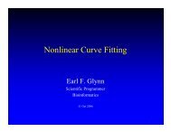
Cusp point. The loci of fold bifurcation in the<br />
parametric plane h, m, drawn as a parametric plot,<br />
are shown in Fig. 1. The two branches join <strong>with</strong><br />
a common tangent at the cusp point. In the vicinity<br />
of this point, the applicable amplitude equation<br />
will include a restriction on deviations of both parameters<br />
that specify the direction of this common<br />
tangent. It can be easily seen that the quadratic<br />
term in the lowest-order Eq. (43) vanishes at y s =2<br />
where the cusp point is located. The equation becomes<br />
trivial at h 2 =2m 2 /e 2 . This relation defines<br />
a direction in the parametric space along which the<br />
second-order deviation is made. The next order deviation<br />
must be orthogonal to this direction. In the
994 L. M. Pismen & B. Y. Rubinstein<br />
h<br />
5<br />
4.75<br />
4.5<br />
0.4<br />
0.6<br />
4.25<br />
5 6 7 8 9 10 11 m<br />
0.5<br />
3.75<br />
3.5<br />
3.25<br />
Fig. 1. Loci of fold and Hopf bifurcation in the parametric plane h, m. The three Hopf curves correspond to g =0.4, 0.5<br />
and 0.6. Solid gray lines show the supercritical, and dashed lines, the subcritical bifurcation. Outside the cusped region, the<br />
unique stationary state suffers oscillatory instability <strong>with</strong>in the loop of the Hopf bifurcation locus. Within the cusped region,<br />
there are three stationary states, of which two, lying on the upper and lower folds of the solution manifold, may be stable.<br />
The solutions on the upper fold are unstable below the Hopf bifurcation line.<br />
vicinity of this point the Landau equation is cast<br />
into (m 3 is set to zero):<br />
∂ 2 a = − e2<br />
6 a3 + m 2 a + e 2 h 3 . (45)<br />
Hopf bifurcation. The dynamical system (42) can<br />
also undergo a Hopf bifurcation. In the operator<br />
<strong>for</strong>m it can be written as:<br />
G(R)u t = f(u) , (46)<br />
where G(R) denotes a capacitance matrix.<br />
The function <strong>Bifurcation</strong>Theory called <strong>for</strong><br />
this type of the problem produces the set (33) of<br />
the amplitude equations (at the Hopf bifurcation<br />
point) <strong>with</strong> the following <strong>for</strong>mulae <strong>for</strong> the coefficients<br />
of the first amplitude equation:<br />
c 2, 1 = U † GU ;<br />
c 2, 2 (R 1 )=−iwU † G R UR 1 . (47)<br />
The Landau coefficient in the second equation is<br />
given by (35) <strong>with</strong> the only replacement of the identity<br />
matrix I by the capacitance matrix G. Expression<br />
<strong>for</strong> the coefficient c 3, 3 (R 1 , R 2 ) of the linear<br />
term is not shown due to its complexity.<br />
We start the computations from the determination<br />
of the Hopf bifurcation manifold. It contains<br />
stationary points of the system at which a matrix<br />
f u −iwG is singular (w denotes the frequency of the<br />
limit cycle). The manifold is given by the following<br />
set of equations:<br />
e y (h − y) − my =0,<br />
e y (g+y−h)+m(1 + g) =0.<br />
These equations are solved to express the values<br />
of the parameters m and h through the stationary<br />
value y = y 0 and the remaining parameter<br />
g = g 0 ; y 0 ,g 0 are thus chosen to parameterize the<br />
2D Hopf bifurcation manifold in the 3D parametric<br />
space:<br />
h = y 0 +<br />
g 0 y 0<br />
y 0 − g 0 − 1 ,<br />
g 0 e y 0<br />
m =<br />
y 0 − g 0 − 1 .<br />
The loci of Hopf bifurcation in the parametric plane<br />
h, m at several chosen values of g are shown in<br />
Fig. 1. Outside the cusped region, the unique stationary<br />
state suffers oscillatory instability <strong>with</strong>in<br />
the loop of the Hopf curve (this is possible at<br />
g
<strong>Computer</strong> <strong>Tools</strong> <strong>for</strong> <strong>Bifurcation</strong> <strong>Analysis</strong> 995<br />
Now it is possible to compute the frequency<br />
w = e y √ 0<br />
y 0 − g 0 y 0 − 1/(1 + g 0 − y 0 )andtheeigenvectors:<br />
{<br />
g(1 − y0 − i √ }<br />
y 0 − g 0 y 0 − 1)<br />
U =<br />
, 1 ;<br />
y 0 (y 0 −1)<br />
y0<br />
4<br />
3.5<br />
3<br />
super<br />
sub<br />
U † =<br />
{<br />
(y 0 − 1) g 0(1 − y 0 + i √ }<br />
y 0 − g 0 y 0 − 1)<br />
,1<br />
1+g 0 −y 0<br />
.<br />
(48)<br />
2.5<br />
2<br />
1.5<br />
1<br />
0.5<br />
sub<br />
As it was done above, one can choose the parametric<br />
deviation of the first-order in such a way as<br />
to make the first amplitude equation trivial. Then<br />
the Landau coefficient in the second equation can<br />
be presented after normalization as:<br />
c 3, 2 /c 3, 1 =(y 0 −g 0 y 0 −1) 3/2 (iy 0 − i<br />
− √ y 0 − g 0 y 0 − 1) −1 e y 0<br />
/12<br />
× (12 − 24g 0 − 24y 0 +40g 0 y 0 −4g 2 0 y 0<br />
+14y 2 0−21g 0 y 2 0 +4g 2 0y 2 0 −2y 3 0 +2g 0 y 3 0<br />
+i √ y 0 −g 0 y 0 −1(−12 + 24g 0 +15y 0<br />
−25g 0 y 0 − 2g 2 0 y 0 − 5y 2 0 +8g 0y 2 0 )) . (49)<br />
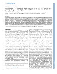
0 0.1 0.2 0.3 0.4 0.5 0.6 0.7<br />
Fig. 2. The stability boundary in the plane (g 0,y 0), separating<br />
the regions of subcritical and supercritical Hopf bifurcation.<br />
The unphysical part of the curve below the boundary<br />
of positive frequency is shown by a dashed line. The solid<br />
circle at g 0 =0.5,y 0= 2 marks the double zero point.<br />
the unphysical part of the curve dipping below the<br />
boundary of positive frequency is shown by a dashed<br />
line. The region of subcritical bifurcations consists<br />
of two disconnected parts, of which the lower one<br />
lies <strong>with</strong>in the region of unique stationary states<br />
and on the lower fold of the solution manifold, and<br />
the upper one, on the upper fold in the region of<br />
multiple solutions.<br />
g0<br />
First, we take note that only a part of the parametric<br />
plane y 0 ,g 0 above the thick solid curve in<br />
Fig. 2 is actually available, since the condition of<br />
positive oscillation frequency requires<br />
y 0 − g 0 y 0 − 1 > 0 . (50)<br />
Within this region, the limit cycle is stable (the bifurcation<br />
is supercritical ) if the real part of the coefficient<br />
at the nonlinear term is negative. Extracting<br />
the real part from (49) brings this condition to the<br />
<strong>for</strong>m<br />
3g 0 +2g 2 0 +2y 0−4g 0 y 0 −2g 2 0 y 0−y 2 0 +2g 0y 2 0 −1<br />
4(y 0 − 1 − g 0 )(y 0 − g 0 y 0 − 1)<br />
< 0 . (51)<br />
Noting that the denominator of the above fraction<br />
is positive whenever the inequality (50) is verified,<br />
one can determine the stability boundary by equating<br />
the numerator in (51) to zero, and combining<br />
the result <strong>with</strong> (50). The stability boundary in the<br />
plane (g 0 ,y 0 ), separating the regions of subcritical<br />
and supercritical bifurcation is shown in Fig. 2;<br />
3. <strong>General</strong> Algorithm<br />
<strong>for</strong> Distributed Systems<br />
3.1. Introduction<br />
The main point of our approach can be <strong>for</strong>mulated<br />
as follows. An algorithm applicable to the nonlinear<br />
analysis of a number of representative realistic<br />
problems must be as general as possible, i.e. it must<br />
be designed <strong>for</strong> classes of problems (say, dynamical<br />
problems, or reaction–diffusion type problems), or<br />
even better, it should embrace all problems which<br />
can be solved using standard methods of bifurcation<br />
expansion.<br />
It is clear that the generalization from particular<br />
problems to some class of such problems can be<br />
per<strong>for</strong>med using an operator <strong>for</strong>m of the problem.<br />
For example, all reaction–diffusion type problems<br />
can be presented in the following operator <strong>for</strong>m:<br />
G(R) ∂ u(r, t)=D(R)(∇·∇)u(r,t)<br />
∂t<br />
+f(u(r,t),R), (52)
996 L. M. Pismen & B. Y. Rubinstein<br />
where ∂/∂t denotes the time differentiation operator,<br />
∇ stands <strong>for</strong> the operator of differentiation over<br />
the spatial variable r; f, u, R are arrays of functions,<br />
variables and bifurcation parameters of the<br />
problem. G(R) andD(R) denote capacitance and<br />
diffusion matrix respectively, which can depend on<br />
the bifurcation parameters.<br />
In its turn problem (52) appears to be a particular<br />
case of most general problem which can be<br />
written as<br />
F(∇, ∂/∂t,u(r,t,R),R)=0, (53)<br />
where F can also include a set of boundary conditions<br />
imposed on the solution u(r, t,R).<br />
3.2. Linear analysis and<br />
dispersion relation<br />
The general standard algorithm <strong>for</strong> derivation of<br />
amplitude equations starts from the linear analysis<br />
of an underlying distributed system in the vicinity<br />
of a basic state. We assume also that <strong>for</strong> each<br />
value R the system admits a stationary spatially<br />
homogeneous solution u 0 (R), which is called basic<br />
state. Typically the basic state becomes unstable<br />
in a certain domain of the parametric space,<br />
and this instability is usually connected <strong>with</strong> the<br />
bifurcations of new solutions <strong>with</strong> a more complicated<br />
spatiotemporal structure. We construct solutions<br />
of the original problem (53) in the <strong>for</strong>m<br />
u = u 0 (R)+ũ(r,t,R), where ũ is a small disturbance<br />
of the basic state. Substituting the solution<br />
in (53) one arrives in the linear approximation in ũ<br />
to the following:<br />
L(∇, ∂/∂t,u 0 (R),R)ũ=0, (54)<br />
where L is a linear operator (Frechet derivative)<br />
calculated at the point u = u 0 acting on small disturbance<br />
ũ. Further on, we shall consider normal<br />
disturbances of the <strong>for</strong>m:<br />
ũ(r, t,R)=A(k,R)exp(σt + ikr) . (55)<br />
The growth rate σ is generally a complex number.<br />
For normal disturbances the evolution equation (54)<br />
is reduced to the eigenvalue problem:<br />
L(ik, σ,u 0 (R),R)A=0, (56)<br />
which usually determines a countable set of<br />
branches of dispersion relation between growth<br />
rates σ n and the wavenumber k = |k|. We assume<br />
that the instability is generated by eigenmodes <strong>with</strong><br />
the growth rates σ j (k, R) =σ jr (k, R)+iω j (k, R).<br />
The conditions σ jr (k, R) = 0 determine instability<br />
boundaries which are called neutral stability curves.<br />
The minima of all functions σ jr (k, R) are reached<br />
at the same value R = R 0 and at (possibly various)<br />
values k = k jc .<br />
If ω j (k jc , R 0 ) = 0, the corresponding instability<br />
is called stationary (monotonous); otherwise,<br />
there is an oscillatory (wavy) instability. In each<br />
of these cases, two possibilities arise depending<br />
on the wavenumber critical value: Either the instability<br />
arises near a nonzero wavenumber k jc<br />
(short-wavelength instability), or the instability domain<br />
is localized around k jc =0(long-wavelength<br />
instability).<br />
The linear analysis procedure also includes determination<br />
of eigenvectors U j , U † j of the linear<br />
problem (56) verifying the equation LU j =0and<br />
its adjoint counterpart L † U † j = 0 needed <strong>for</strong> further<br />
calculations. Setting aside most complicated<br />
cases of double and triple bifurcation points we,<br />
however, permit simple degenerate cases, when each<br />
instability mode is characterized by a unique set of<br />
wavevector and frequency values.<br />
A general solution u l of the linear problem (54)<br />
can be written as a superposition of several normal<br />
modes <strong>with</strong> jth mode characterized by its scalar<br />
amplitude a j , particular values of the wavevector<br />
k j , time frequency ω j , eigenvector of the mode U j<br />
anditsorderofsmallnessd j :<br />
N∑<br />
u l =ε d 0<br />
a 0 U 0 + ε d j<br />
(a j U j exp(ik j r 0 + iω j t 0 )<br />
j=1<br />
+ a ∗ j Ũj exp(−ik j r 0 − iω j t 0 )) , (57)<br />
where ∗ denotes an operation of the complex conjugation<br />
and ˜ denotes an operation of Dirac conjugation,<br />
which in the case of real vector function<br />
F is reduced to the standard complex conjugation.<br />
The coefficient a 0 ≠ 0 if monotonic long-scale mode<br />
characterized by the zero value of the wavenumber<br />
and time frequency is permitted. Each mode gives<br />
rise to a corresponding solvability condition which<br />
determines a slow spatiotemporal dynamics of the<br />
mode’s amplitude using the consequent orders of<br />
the multiscale expansion of the problem.<br />
3.3. Multiscale expansion<br />
In order to simplify derivations, we shall eliminate<br />
trivial parametric dependence of the basic state by
<strong>Computer</strong> <strong>Tools</strong> <strong>for</strong> <strong>Bifurcation</strong> <strong>Analysis</strong> 997<br />
trans<strong>for</strong>ming to a new variable û = u−u 0 (R). The<br />
resulting system, F(∇, ∂/∂t,û+u 0 ,R)=0hasthe<br />
same <strong>for</strong>m as (53) but contains a modified operator<br />
ˆF(∇, ∂/∂t,û,R)=F(∇,∂/∂t,û+u 0 ,R). Since,<br />
by definition, u 0 satisfies F(∇, ∂/∂t,u 0 ,R)=0,<br />
û= 0 is a zero of ˆF(∇, ∂/∂t,û,R). Now we can<br />
drop the hats over the symbols and revert to the<br />
original <strong>for</strong>m (53) while keeping in mind that u =0<br />
is a stationary solution <strong>for</strong> all R and, consequently,<br />
all derivatives F R , F RR , etc. computed at u =0<br />
vanish.<br />
We use the expansions (2) <strong>for</strong> variables and parameters<br />
and introduce a hierarchy of time scales<br />
t k , thus replacing the function u by a function of<br />
an array of rescaled time variables. Accordingly,<br />
the time derivative is expanded as in (3). The spatial<br />
derivative is expanded similarly:<br />
∇ = ∇ 0 + ε α ∇ 1 , (58)<br />
where α denotes the spatial scaling which depends<br />
on a particular problem; <strong>for</strong> the sake of simplicity,<br />
we shall use only positive integer values of α. Substituting<br />
expansions (2) and (3) and (58) into the<br />
original problem (53) and expanding in ε, onearrives<br />
at a set of equations <strong>for</strong> different orders of ε.<br />
In the lowest-order we reproduce the equation<br />
F(∇ 0 ,∂ 0 ,u 0 ,R 0 ) = 0 determining the basic solution<br />
computed at the critical values of bifurcation<br />
parameters. In the next order the linear problem<br />
(54) is reproduced in the following <strong>for</strong>m:<br />
F u (∇ 0 ,∂ 0 ,u 0 ,R 0 )u 1 =0. (59)<br />
The solution u 1 consists of normal modes <strong>with</strong><br />
d j =1.<br />
In the consequent orders one arrives at the<br />
equations of the <strong>for</strong>m:<br />
F u (∇ 0 ,∂ 0 ,u 0 ,R 0 )u n =g n , (60)<br />
where g n denotes the nth order inhomogeinity vector.<br />
A set of solvability conditions <strong>for</strong> each of the<br />
normal modes appearing in the linear solution (57)<br />
will define slow spatiotemporal dynamics of the amplitude<br />
of each mode. It can be shown that only<br />
part of the inhomogeinity g n which projects on<br />
the principal harmonic of a certain mode will contribute<br />
to the corresponding solvability condition.<br />
Denoting the scalar product by angle brackets and<br />
the projection operator on the harmonic exp(iβ)<br />
as P(·, exp(iβ)), one can write the solvability condition<br />
<strong>for</strong> jth normal mode in the nth order as<br />
follows:<br />
〈U † j , P(g n,e ik jr 0 +iω j t 0<br />
)〉 =0, (61)<br />
where U † j denotes the eigenvector of the adjoint linear<br />
problem L † U † j = 0 corresponding to the jth<br />
mode.<br />
The linear inhomogeneous problem (60) must<br />
be solved <strong>with</strong> respect to u n provided solvability<br />
conditions (61) are satisfied. To this particular solution<br />
of (60) one must add a linear solution term<br />
of the corresponding order of smallness. The combined<br />
solution is used <strong>for</strong> the calculations of the<br />
next order inhomogeinity g n+1 .<br />
In the second-order the vector of inhomogeinity<br />
g 2 can be represented in the <strong>for</strong>m:<br />
g 2 = − 1 2 F uu(∇ 0 ,∂ 0 ,u 0 ,R 0 )u 1 u 1<br />
−F uR (∇ 0 ,∂ 0 ,u 0 ,R 0 )u 1 R 1<br />
−δ α, 1 F u∇ (∇ 0 ,∂ 0 ,u 0 ,R 0 )∇ 1 u 1<br />
−F u<br />
∂ (∇ 0 ,∂ 0 ,u 0 ,R 0 )∂ 1 u 1 , (62)<br />
∂t<br />
where the Kronecker symbol δ α, β = 0 at α ≠ β<br />
and δ α, α = 1. The resulting set of the conditions in<br />
the second-order is resolved further <strong>with</strong> respect to<br />
the derivative of the amplitudes ∂ 1 a j . This result<br />
presents the set of the amplitude equations of the<br />
second-order and in its turn is used <strong>for</strong> derivation<br />
of the amplitude equations in the next orders.<br />
The final result is the set of the amplitude equations<br />
written in most general <strong>for</strong>m which is valid <strong>for</strong><br />
the combination of the normal modes in (57) and<br />
specified value of the spatial variable scaling exponent<br />
α. This set further can be “projected” onto<br />
a particular class of the problems to produce a required<br />
<strong>for</strong>mula. These <strong>for</strong>mulae are applicable to<br />
any problem from the selected class. In order to<br />
make actual calculations <strong>for</strong> a particular problem<br />
one must determine the values of the wavevectors,<br />
frequency, eigenvectors, etc. and substitute them<br />
into the abovementioned <strong>for</strong>mulae.<br />
3.4. Function <strong>Bifurcation</strong>Theory<br />
The function <strong>Bifurcation</strong>Theory used <strong>for</strong> derivation<br />
of the normal <strong>for</strong>ms <strong>for</strong> dynamical systems<br />
can be applied <strong>with</strong> some additions to distributed<br />
systems.
998 L. M. Pismen & B. Y. Rubinstein<br />
If it is required to derive the normal <strong>for</strong>m <strong>for</strong><br />
a single mode arising at a bifurcation point of the<br />
distributed system, one may use the call<br />
<strong>Bifurcation</strong>Theory[operatoreqn, u, R, t,<br />
{r, dim}, spatscale, {U, U † },<br />
amp, coef, eps, order, wavenumber, freq,<br />
opts].<br />
Here r denotes a spatial variable (that can be a<br />
vector); dim is the space dimension and spatscale<br />
denotes an array consisting of the name of the spatial<br />
variable and its (integer) scaling exponent α.<br />
Finally, wavenumber must be set equal to zero <strong>for</strong><br />
a long-scale instability and to some symbol in the<br />
short-scale case. In the latter case the wavevector<br />
needed <strong>for</strong> the calculations is generated automatically.<br />
The differentiation operators ∂/∂t and ∇<br />
used in the operator equation operatoreqn are represented<br />
by the symbols Nabla[t] and Nabla[r],<br />
respectively.<br />
A more complicated <strong>for</strong>m must be used in a case<br />
when there is an angular degeneracy of the normal<br />
modes, namely, when the different modes have the<br />
same values of their parameters but the wavevectors<br />
<strong>with</strong> equal lengths have different directions. It is rational<br />
to specify the mode data using the angular<br />
measurment <strong>for</strong> the wavevectors —<br />
<strong>Bifurcation</strong>Theory[operatoreqn, u, R, t,<br />
{r, dim}, spatscale, {U, U † },<br />
amps, coef, eps, order, wavenumber, freq,<br />
ampout, opts],<br />
where amps consists of the pairs {a j ,β j }<strong>with</strong> β j<br />
denoting an angle between the wavevector of the<br />
jth mode a j and some selected direction. If the<br />
argument ampout specifying the names of the amplitudes<br />
<strong>for</strong> which equations must be generated is<br />
omitted, equations <strong>for</strong> first amplitude only from the<br />
array amps would be produced.<br />
The most general <strong>for</strong>m of the function is used<br />
<strong>for</strong> algebraically degenerated cases:<br />
<strong>Bifurcation</strong>Theory[operatoreqn, u, R, t,<br />
{r, dim}, spatscale, amps,<br />
coef, eps, order, ampout, options]<br />
derives a set of amplitude equations <strong>for</strong> a distributed<br />
system of partial differential equations<br />
writteninanoperator<strong>for</strong>m.Hereamps is an array<br />
of elements specifying the normal modes appearing<br />
in the linear solution (57). Each item of amps is<br />
an array of six elements in the following order —<br />
amplitude of the mode (a j ), mode wavevector (k j ),<br />
time frequency (ω j ), eigenvector (U j ), eigenvector<br />
of the adjoint problem (U † j ),andorderofsmallness<br />
of the normal mode (d j ). ampout again denotes an<br />
array of the amplitude names <strong>for</strong> which the amplitude<br />
equations must be generated.<br />
4. Amplitude Equations <strong>for</strong><br />
Reaction–Diffusion Problems<br />
4.1. Long-scale instabilities<br />
In this and the next subsections we present the result<br />
of derivation of the amplitude equations <strong>for</strong><br />
reaction–diffusion problem (52) <strong>with</strong> capacitance<br />
matrix G equal to identity matrix I and diffusivity<br />
matrix D which does not depend on the bifurcation<br />
parameters.<br />
We start from the case where the instability domain<br />
is localized around k c = 0 restricting ourselves<br />
to nondegenerated nonresonant cases.<br />
The operator equation corresponding to the<br />
problem may be written as:<br />
DD.(Nabla[r] . Nabla[r])∗∗u + f[u, R] -<br />
Nabla[t]∗∗u == 0<br />
where DD denotes the diffusivity matrix. Operator<br />
Nabla[r] is assumed to be vectorial, hence the<br />
scalar Laplacian is written as scalar product of two<br />
differential operators. The function is called as<br />
follows:<br />
<strong>Bifurcation</strong>Theory[<br />
DD.(Nabla[r].Nabla[r])**u + f[u,R] -<br />
Nabla[t]**u == 0,<br />
u, R, t, {r,2},{r,1},{U,Ut}, a, c, eps, 2,<br />
0, 0]<br />
Un<strong>for</strong>tunately, the version 2.2.2 of Mathematica<br />
used in development of the package has no perfect<br />
typesetting abilities like the version 3.0. As<br />
a result the output of the function is very lengthy<br />
and is difficult to understand <strong>for</strong> the inexperienced<br />
user. Here and further, we present output produced<br />
by the function <strong>Bifurcation</strong>Theory using standard<br />
textbook notation.<br />
The result produced by the function coincides<br />
<strong>with</strong> that of the monotonic bifurcation of the dynamical<br />
system (36) <strong>with</strong> the only exception — the<br />
Landau equation is converted into the Ginzburg–<br />
Landau equation <strong>with</strong> an additional diffusional<br />
term of the <strong>for</strong>m:<br />
U † DU<br />
U † U (∇ 1∇ 1 )a. (63)
<strong>Computer</strong> <strong>Tools</strong> <strong>for</strong> <strong>Bifurcation</strong> <strong>Analysis</strong> 999<br />
Now we turn to the case of the Hopf bifurcation<br />
<strong>for</strong> the same problem. The last argument of the<br />
function <strong>Bifurcation</strong>Theory denoting the limit cycle<br />
frequency now is set to w rather than zero:<br />
<strong>Bifurcation</strong>Theory[<br />
DD.(Nabla[r].Nabla[r])**u + f[u,R] -<br />
Nabla[t]**u == 0,<br />
u, R, t, {r,2},{r,1},{U,Ut}, a, c, eps, 2,<br />
0, w]<br />
As in the previous case the resulting set of equations<br />
is given by (33) <strong>with</strong> the addition of the same<br />
diffusional term.<br />
4.2. Turing bifurcation<br />
Short-scale instabilities are characterized by a<br />
nonzero value of the wavenumber; hence, several<br />
modes <strong>with</strong> different directions of the wavevector<br />
are permitted.<br />
This case is characterized by the nonzero value<br />
of the wavenumber and zero frequency, what is reflected<br />
in the function is called:<br />
<strong>Bifurcation</strong>Theory[<br />
DD.(Nabla[r].Nabla[r])**u + f[u,R] -<br />
Nabla[t]**u == 0,<br />
u, R, t, {r,2},{r,1},{U,Ut},<br />
{{a1,0}, {a2, alpha}}, c, eps, 2, k, 0]<br />
It corresponds to the case of two normal modes <strong>with</strong><br />
awavenumberequaltok— a wavevector k 1 of the<br />
first mode a 1 is directed along the x-axis in a plane<br />
(the dimension of spatial variable is set equal to<br />
2); the wavevector k 2 of the second mode a 2 makes<br />
the angle α <strong>with</strong> k 1 . We assume that this angle is<br />
not equal to π/3 or2π/3 inordertomakethese<br />
two modes nonresonant. The argument specifying<br />
names of the amplitudes <strong>for</strong> output is omitted, so<br />
the equations <strong>for</strong> amplitude a 1 are only generated<br />
by default.<br />
Theresultmaybewrittenas:<br />
∂ 1 a 1 = c 2,1,1<br />
c 2,2<br />
(ik 1 ∇ 1 )a 1 + c 2,3(R 1 )<br />
c 2,2<br />
a 1 ,<br />
∂ 2 a 1 = c 3,4<br />
c 3,3<br />
|a 2 | 2 a 1 + c 3,5<br />
c 3,3<br />
|a 1 | 2 a 1<br />
+ c 3,6(R 1 ,R 2 )<br />
c 3,3<br />
a 1 + c 3,1,1<br />
c 3,3<br />
(∇ 1 ∇ 1 )a 1<br />
(64)<br />
+ c 3,1,2<br />
c 3,3<br />
(ik 1 ∇ 1 ) 2 a 1 + c 3,2,1(R 1 )<br />
c 3,3<br />
(ik 1 ∇ 1 )a 1 .<br />
The coefficients c 2, 2 = c 3, 3 = U † U determine<br />
a normalization of the eigenvectors.<br />
For the first time scale t 1 we have a linear equation.<br />
Its linear term coefficient is proportional to<br />
the first-order deviation of the bifurcation parameter<br />
vector and is given by (26). The differential<br />
term has a coefficient of the <strong>for</strong>m<br />
c 2, 1, 1 =2U † DU . (65)<br />
Choosing the parametric deviation R 1 one may set<br />
the real part of the linear term coefficient equal to<br />
zero; then the resulting equation will admit a traveling<br />
wave solution.<br />
The Ginzburg–Landau equation at the slower<br />
time scale is most interesting. It contains two nonlinear<br />
terms describing interaction between the two<br />
modes as well as the self-interaction of the principal<br />
mode a 1 . Interaction coefficient c 3, 4 of two modes<br />
depends on the angle α between their wavevectors<br />
and is calculated using the <strong>for</strong>mula:<br />
c 3, 4 = −U † f uu UR(f u )f uu UŨ<br />
− U † f uu UR(f u − 2k 2 D(1 − cos α))f uu UŨ<br />
− U † f uu ŨR(f u − 2k 2 D(1 + cos α))f uu UU<br />
+ U † f uuu UUŨ . (66)<br />
The self-interaction coefficient c 3, 5 may be<br />
found as half of the value of c 3, 4 calculated at α =0:<br />
c 3,5 =−U † f uu UR(f u )f uu UŨ<br />
− U † f uu ŨR(f u − 4k 2 D)f uu UU/2<br />
+ U † f uuu UUŨ/2 . (67)<br />
The linear term coefficient is supplied by (63)<br />
<strong>with</strong> replacement of R(f u − iwI) byR(−k 2 D+f u ).<br />
There are three diffusional terms in the<br />
Ginzburg–Landau equation; one is given by (63),<br />
another term coefficient c 3, 2, 1 depends on the parametric<br />
deviation of the first-order and usually<br />
can be removed by the appropriate choice of this<br />
deviation:<br />
c 3, 2, 1 (R 1 )<br />
=2(U † R(−k 2 D+f u )f uR UR 1 )(U † DU)/(U † U)<br />
− 2U † DR(−k 2 D+f u )f uR UR 1<br />
+2(U † R(−k 2 D+f u )DU)(U † f uR UR 1 )/(U † U)<br />
+2U † f uR R(−k 2 D+f u )DUR 1 . (68)
1000 L. M. Pismen & B. Y. Rubinstein<br />
The coefficient c 3, 1, 2 independent of the parametric<br />
deviation has the following <strong>for</strong>m:<br />
c 3, 1, 2 =4(U † R(−k 2 D+f u )DU)(U † DU)/(U † U)<br />
− 4U † DR(−k 2 D + f u )DU . (69)<br />
4.2.1. Hopf bifurcation<br />
Now we turn to the case of the Hopf bifurcation <strong>for</strong><br />
the same problem. The resulting set of equations<br />
is given by (65) <strong>with</strong> slightly changed <strong>for</strong>mulae <strong>for</strong><br />
the coefficients in the Ginzburg–Landau equation.<br />
The modes interaction coefficient c 3, 4 is calculated<br />
as shown in (66) <strong>with</strong> the only replacement of<br />
R(f u −2k 2 D(1+cos α)) by R(f u −2k 2 D(1+cos α)−<br />
2iwI), where I stands <strong>for</strong> the identity matrix. Similarly,<br />
in the expression (67) <strong>for</strong> the self-interaction<br />
coefficient one must replace R(f u −4k 2 D)byR(f u −<br />
4k 2 D−2iwI).<br />
The linear term coefficient again is supplied by<br />
(39) <strong>with</strong> the replacement of R(f u )byR(f u −k 2 D−<br />
iwI).<br />
The diffusional coefficient c 3, 2, 1 depending on<br />
the parametric deviation is found as (69) <strong>with</strong> the<br />
replacement of R(f u − k 2 D)byR(f u −k 2 D−iwI).<br />
The same replacement is valid <strong>for</strong> another diffusional<br />
coefficient c 3, 1, 2 .<br />
In order to per<strong>for</strong>m calculation of the coefficients<br />
of the amplitude equations describing slow<br />
dynamics in the vicinity of a bifurcation point of<br />
a particular problem, values of all elements of the<br />
output of the function <strong>Bifurcation</strong>Theory need to<br />
be specified, substitute them into the <strong>for</strong>mulae and<br />
make a simplification if needed. In this section we<br />
illustrate the usage of the above results using two<br />
simple models.<br />
4.3. Brusselator model<br />
The first example is a well-known Brusselator model<br />
[Nicolis & Prigogine, 1977] of chemical oscillations:<br />
∂z/∂t = a − (1 + b)z + uz 2 +(∇∇)z,<br />
∂u/∂t = bz − uz 2 + d(∇∇)u.<br />
The variables u, z denote concentrations of the “activator”<br />
and “inhibitor” species. This system always<br />
has a unique stationary homogeneous solution<br />
z = a, u = b/a. The dispersion relation is found as<br />
follows:<br />
a 2 + a 2 k 2 + dk 2 − bdk 2 + dk 4<br />
+ iw(1 + a 2 − b + k 2 + dk 2 ) − w 2 =0<br />
Now we can trace two possibilities — the first is <strong>for</strong><br />
monotonic bifurcation <strong>with</strong> frequency w =0and<br />
the second <strong>for</strong> Hopf bifurcation <strong>with</strong> nonzero w.<br />
4.3.1. Monotonic bifurcation<br />
We start from the determination of the bifurcation<br />
curve describing a dependence of the bifurcation parameter<br />
b on the wavenumber k and then we find the<br />
minimum of this curve b cm =(1+a/ √ d) 2 reached<br />
at k cm =(a 2 /d) 1/4 .<br />
It can be seen that the monotonic bifurcation<br />
corresponds to the short-scale instability. The<br />
eigenvectors of the problem can be found as:<br />
{ } ad<br />
U =<br />
a + √ d , 1 ;<br />
{ √ }<br />
(70)<br />
a + d<br />
U † = , 1 .<br />
a<br />
Calculation of the coeffcients of amplitude<br />
equations (65) shows that the coefficient c 211 of the<br />
linear differential term in the first equation is equal<br />
to zero identically, the linear term is proportional<br />
to the bifurcation parameter deviation b 1 :<br />
d √ db 1<br />
∂ 1 a 1 = −<br />
(a + √ d)(1 − d) a 1 .<br />
Setting b 1 = 0 we can trivialize the above equation.<br />
In the next order equation some of the coefficients<br />
vanish: c 3, 2, 1 (0) = 0; c 3, 1, 1 =0.The coefficient<br />
of the only nonzero diffusional term in (65) is<br />
given by:<br />
4d 2<br />
c 3, 1, 2 =<br />
a(a + √ d) ,<br />
the linear term coefficient is proportional to secondorder<br />
parametric deviation:<br />
c 3, 6 (R 2 )=− d√ db 2<br />
a + √ d .<br />
The dependence of the modes interaction coefficient<br />
on α is provided by:<br />
2d 2<br />
c 3, 4 =<br />
a(a + √ d) 2 (4 cos 2 α − 1) 2<br />
× (−8a 3 +7a 2√ d+18ad − 8d √ d<br />
+2a 2√ d(−2cos2α+cos4α)<br />
+4ad(4 cos 2α +cos4α)) .<br />
(71)
<strong>Computer</strong> <strong>Tools</strong> <strong>for</strong> <strong>Bifurcation</strong> <strong>Analysis</strong> 1001<br />
It can be easily seen that this coefficient diverges<br />
at cos α = ±1/2, i.e. at α = π/3, 2π/3. The<br />
reason of the divergence is the existence of the resonance<br />
between the two modes, and <strong>for</strong> proper description<br />
one needs to incorporate the third mode<br />
<strong>with</strong> a wavevector k 3 such that k 1 + k 2 + k 3 =0.<br />
The resonant cases are considered below. Finally<br />
we present the self-interaction coefficient:<br />
c 3, 5 =<br />
d 2<br />
9a(a + √ d) 2 (−8a3 +5a 2√ d+38ad−8d √ d) .<br />
4.3.2. Oscillatory bifurcation<br />
(72)<br />
The minimum of the bifurcation curve b co =1+a 2<br />
is found at k co = 0, which means that the oscillatory<br />
bifurcation <strong>with</strong> frequency of the limit cycle is<br />
w = a that corresponds to the long-scale instability.<br />
The eigenvectors of the problem can be found as:<br />
{<br />
U = −<br />
a }<br />
a − i , 1 ;<br />
U † =<br />
{ a + i<br />
a , 1 }<br />
. (73)<br />
The calculation produces Eqs. (33) <strong>with</strong> coefficients<br />
given by (40) and (42) <strong>with</strong> the additional<br />
diffusional term <strong>with</strong> coefficient equal to<br />
((d +1)+ia(d − 1))/2.<br />
It can also be noted here that by equating the<br />
critical values of the bifurcation parameter b <strong>for</strong><br />
monotonic and oscillatory cases it is possible to find<br />
the critical value a c =2 √ d/(d − 1) at which the bifurcation<br />
is degenerate, i.e. both Hopf and Turing<br />
modes are permitted. This degenerate case will be<br />
described below.<br />
4.4. Two-level laser model<br />
The simple model of a two-level laser [Coullet et al.,<br />
1989] describes the dynamics of the electric field interacting<br />
<strong>with</strong> an active media. The model equations<br />
are the following:<br />
A t = ia(∇∇)A + σ(P − A) ,<br />
P t =(1+iΩ)P − (R − n)A, (74)<br />
n t = −bn +1/2(A ∗ P + AP ∗ ) .<br />
The variables A, P, n denote complex amplitude<br />
of the electrical field, complex media polarization<br />
density and real atomic population inversion,<br />
respectively.<br />
This model exhibits short-scale oscillatory instability<br />
in the vicinity of the basic nonlasing solution<br />
A 0 = P 0 = n 0 = 0. It must be noted that in<br />
order to make calculations one need to complete the<br />
system (75) <strong>with</strong> complex conjugation of first two<br />
equations <strong>for</strong> A ∗ ,P ∗ . As a result the state vector<br />
{A, A ∗ ,P,P ∗ ,n}appears to have five components<br />
instead of the original three.<br />
4.4.1. Oscillatory bifurcation<br />
The bifurcation curve has a <strong>for</strong>m:<br />
( )<br />
Ω−ak<br />
2 2<br />
R =1+<br />
. (75)<br />
1+σ<br />
The lowest minimum (<strong>for</strong> positive a and Ω)<br />
of this curve lies at k c = √ Ω/a and it equals to<br />
R 0 = 1, the critical frequency w c = Ω. The eigenvectors<br />
of the problem are given by:<br />
U = {0, 1, 0, 1, 0} ; U † =<br />
{0, 1 }<br />
σ , 0, 1, 0 .<br />
(76)<br />
In this case one does not need to shift the basic<br />
solution because it does not depend on the parameters<br />
of the problem. For the calculation of<br />
the coefficients of the amplitude equations in this<br />
case one needs additional preparatory step due to<br />
the complex nature of the original problem. In the<br />
<strong>for</strong>mulae <strong>for</strong> the coefficients <strong>for</strong> short-scale instabilities<br />
one may find the notion Ũ denoting the<br />
so-called Dirac conjugated eigenvector U. These<br />
vectors present particular values of the state vector,<br />
which in our case has two complex conjugated<br />
variable components. The construction of the vector<br />
Ũ out of U may be written symbolically in the<br />
<strong>for</strong>m:<br />
Ũ = G(U ∗ ) , (77)<br />
where ∗ denotes usual complex conjugation and<br />
G is an operation of mutual interchange of the vector<br />
components corresponding to the complex conjugated<br />
variables. In our case the complex conjugated<br />
variables A, A ∗ have to be the first positions<br />
in the state vector, while P, P ∗ are at the next<br />
two places. As a result the vector Ũ is constructed<br />
as:<br />
Ũ = {1, 0, 1, 0, 0} .<br />
The lowest-order equation <strong>for</strong> one of two excited<br />
modes <strong>with</strong> amplitudes a 1 , a 2 and wavevectors
1002 L. M. Pismen & B. Y. Rubinstein<br />
k 1 , k 2 is written as:<br />
∂ 1 a 1 =2a(k 1 ∇ 1 )a 1 + σa 1R 1<br />
1+σ , (78)<br />
and may be simplified by setting R 1 =0.<br />
It appears that the term describing the mode–<br />
mode interaction in the Ginzburg–Landau equation<br />
in our case does not depend on the value of the angle<br />
between mode wavevectors and is given by c 3, 4 =<br />
−2/b; the self-interaction coefficient c 3, 5 = −1/b.<br />
Two out of three diffusional coefficients in the second<br />
amplitude equation are not zeros:<br />
c 3, 1, 1 = − ia σ ;<br />
c 4a 2<br />
3, 1, 2 = −<br />
(1 + σ)(1 + σ − iΩ) .<br />
(79)<br />
Finally the amplitude equation may be written in<br />
the <strong>for</strong>m:<br />
σ<br />
∂ 2 a 1 = −<br />
b(1 + σ) (2|a 2| 2 + |a 1 | 2 )a 1<br />
−<br />
−<br />
4a 2<br />
(1 + σ)(1 + σ − iΩ) (k 1∇ 1 ) 2 a 1<br />
ia<br />
1+σ (∇ 1∇ 1 )a 1 + σR 2<br />
(1 + σ) a 1 . (80)<br />
5. Amplitude Equations <strong>for</strong><br />
Convective Problems<br />
5.1. Convective instabilities<br />
The convective problems are characterized by the<br />
presence of the additional convective term in<br />
Eq. (52) and can be written in the following <strong>for</strong>m<br />
[Rovinsky & Menzinger, 1992, 1993]:<br />
∂<br />
u(r, t)=D(∇·∇)u(r,t)+εV(n·∇)u(r,t)<br />
∂t<br />
+f(u(r,t),R), (81)<br />
where n denotes a constant vector determining the<br />
direction of flow and the matrix V sets the velocities<br />
values; it is assumed that the velocities are<br />
of the order ε. Then <strong>for</strong> the Turing instability<br />
one must call the function <strong>Bifurcation</strong>Theory as<br />
follows:<br />
<strong>Bifurcation</strong>Theory[<br />
DD.(Nabla[r].Nabla[r])**u + f[u,R] +<br />
eps V.({1,0}.Nabla[r])**u -<br />
Nabla[t]**u == 0,<br />
u, R, t, {r,2},{r,1},{U,Ut},<br />
{{a1,0}, {a2, alpha}}, c, eps, 2, k, 0]<br />
Here the velocity direction is chosen parallel to the<br />
x-axis. Note that the small parameter of expansion<br />
eps in this case appears explicitly in the operator<br />
equation describing the problem. The result produced<br />
may be written as:<br />
∂ 1 a 1 = c 2, 1, 1<br />
c 2, 2<br />
(ik 1 ∇ 1 )a 1 + c 2, 3<br />
c 2, 2<br />
a 1 + c 2, 3(R 1 )<br />
c 2, 2<br />
a 1 ,<br />
∂ 2 a 1 = c 3, 4<br />
c 3, 3<br />
|a 2 | 2 a 1 + c 3, 5<br />
c 3, 3<br />
|a 1 | 2 a 1 + c 3, 6<br />
c 3, 3<br />
a 1<br />
+ c 3, 6(R 1 , R 2 )<br />
c 3, 3<br />
a 1 + c 3, 1, 1<br />
c 3, 3<br />
(∇ 1 ∇ 1 )a 1<br />
+ c 3, 1, 2<br />
c 3, 3<br />
(ik 1 ∇ 1 ) 2 a 1 + c 3, 2, 1<br />
c 3, 3<br />
(ik 1 ∇ 1 )a 1<br />
(82)<br />
+ c 3, 2, 1(R 1 )<br />
c 3, 3<br />
(ik 1 ∇ 1 )a 1 + c 3, 2, 2<br />
c 3, 3<br />
(n∇ 1 )a 1 .<br />
It can be noted that the set of equations is very<br />
similar to Eq. (65) <strong>with</strong> the addition of some terms.<br />
Here we write the expressions <strong>for</strong> the coefficients<br />
which are changed or added comparing <strong>with</strong> coefficients<br />
of (65). The additional linear term in the<br />
first equation is due to the velocity matrix V and<br />
its coefficient is given by:<br />
c 2, 3 = ikU † VU .<br />
Similarly, there are two linear terms in the second<br />
equation, their coefficients now depend on V:<br />
c 3, 6 = k 2 U † VR(f u − k 2 D)VU − k 2 (U † VR(f u − k 2 D)VU)(U † VU)/(U † U) ,<br />
c 3, 6 (R 1 , R 2 )=(U † R(f u −k 2 D)f uR UR 1 )(U † f uR UR 1 )/(U † U)+U † f uR UR 2<br />
− U † f uR R(f u − k 2 D)f uR UR 1 R 1 + U † f uRR UR 1 R 1 /2<br />
(83)<br />
− ikU † VR(f u − k 2 D)f uR UR 1 + ik(U † VR(f u − k 2 D)f uR UR 1 )(U † VU)/(U † U)<br />
+ ik(U † VR(f u − k 2 D)VU)(U † f uR UR 1 )/(U † U) − ikU † f uR R(f u − k 2 D)VUR 1 .
There is also additional differential term <strong>with</strong> the coefficient given by:<br />
<strong>Computer</strong> <strong>Tools</strong> <strong>for</strong> <strong>Bifurcation</strong> <strong>Analysis</strong> 1003<br />
c 3, 2, 1 =2ik(U † R(−k 2 D + f u )VU)(U † DU)/(U † U) − 2ikU † DR(−k 2 D + f u )VU<br />
+2ik(U † R(−k 2 D + f u )DU)(U † VU)/(U † U) − 2ikU † VR(−k 2 D + f u )DU . (84)<br />
The long-scale Hopf instability case is solved by following lines:<br />
<strong>Bifurcation</strong>Theory[<br />
DD.(Nabla[r].Nabla[r])**u + f[u,R] +<br />
eps V.({1,0}.Nabla[r])**u- Nabla[t]**u == 0,<br />
u, R, t, {r,2},{r,1},{U,Ut}, a, c, eps, 2, 0, w]<br />
The resulting Ginzburg–Landau equation reads:<br />
∂ 2 a = c 3, 4<br />
c 3, 3<br />
|a| 2 a + c 3, 5(R 1 , R 2 )<br />
c 3,3<br />
a + c 3, 1, 1<br />
c 3, 3<br />
(∇ 1 ∇ 1 )a + c 3, 2, 1<br />
c 3, 3<br />
(n∇ 1 )a. (85)<br />
Here are the coefficients of the equation:<br />
c 3, 3 = U † U ,<br />
c 3, 4 = U † f uuu UUŨ/2 − U† f uu UR(f u )f uu UŨ<br />
− U † f uu ŨR(f u − 2iwI)f uu UU/2 ,<br />
c 3, 1, 1 = U † DU ,<br />
c 3, 2, 1 = U † VU . (86)<br />
The linear term coefficient c 3, 5 (R 1 ) is given by<br />
Eq. (36).<br />
6. Resonant and Degenerate Cases<br />
In this section we review the most difficult cases of<br />
bifurcation analysis — resonant and algebraically<br />
degenrate bifurcations of distributed systems. We<br />
consider the three-mode resonance in the reaction–<br />
diffusion problem and demonstrate the ability of the<br />
function <strong>Bifurcation</strong>Theory to cope <strong>with</strong> degenerate<br />
case of simultaneous existence of the Hopf and<br />
Turing bifurcations. A simple example of calculation<br />
of the amplitude equation coefficients <strong>for</strong> Brusselator<br />
model is presented. Some nontrivial examples<br />
of usage the function <strong>Bifurcation</strong>Theory <strong>for</strong><br />
description of resonant patterns in nonlinear optics<br />
are found in [Rubinstein & Pismen, 1997, 1998].<br />
6.1. Three-wave resonance in<br />
turing bifurcation<br />
The short-scale instabilities can demonstrate resonance<br />
of normal modes, i.e. resonance of their frequencies<br />
w j and wavevectors k j :<br />
∑<br />
w j =0;<br />
j<br />
∑<br />
j<br />
k j =0. (87)<br />
The maximal number of the resonant modes is not<br />
limited, the minimal is equal to three. The simplest<br />
resonant situation arises <strong>with</strong> three monotonic<br />
modes <strong>with</strong> the wavevectors k j satisfying the condition:<br />
k 1 + k 2 + k 3 = 0, i.e. the angle between the<br />
adjacent modes is 2π/3. If two out of these three<br />
modes are chosen, calculations show that the coefficient<br />
of the modes interaction term given by (66)<br />
diverges [cf. Eq. (72)], and, hence, the third mode<br />
must be incorporated in order to describe the resonance<br />
properly.<br />
6.1.1. <strong>General</strong> results<br />
The function <strong>Bifurcation</strong>Theory enables to generate<br />
the normal <strong>for</strong>ms <strong>for</strong> resonances, in this case<br />
the values of the angles specifying the directions of<br />
the wavevectors must be set explicitly:<br />
<strong>Bifurcation</strong>Theory[<br />
DD.(Nabla[r].Nabla[r])**u + f[u,R] -<br />
Nabla[t]**u == 0,<br />
u, R, t, {r,2},{r,1},{U,Ut},<br />
{{a1,0}, {a2, 2 Pi/3}, {a3, 4 Pi/3}}, c,<br />
eps, 2, k, 0]<br />
Here we present the results produced by the function<br />
<strong>Bifurcation</strong>Theory <strong>for</strong> the three modes resonance.<br />
These <strong>for</strong>mulae may appear helpful <strong>for</strong> calculations<br />
even “by hand”.
1004 L. M. Pismen & B. Y. Rubinstein<br />
The normal <strong>for</strong>ms <strong>for</strong> the amplitude a 1 is given by (54) <strong>with</strong> additional resonant terms:<br />
∂ 1 a 1 = c 2, 1, 1<br />
c 2, 2<br />
(ik 1 ∇ 1 )a 1 + c 2, 4(R 1 )<br />
c 2, 2<br />
a 1 + c 2, 3<br />
c 2, 2<br />
a ∗ 2 a∗ 3 ,<br />
∂ 2 a 1 = c 3, 7<br />
c 3, 5<br />
|a 3 | 2 a 1 + c 3, 9<br />
c 3, 5<br />
|a 2 | 2 a 1 + c 3, 11<br />
c 3, 5<br />
|a 1 | 2 a 1 + c 3, 6(R 1 )<br />
c 3, 5<br />
a ∗ 2 a∗ 3 + c 3, 12(R 1 , R 2 )<br />
c 3, 5<br />
a 1<br />
+ c 3, 1, 1<br />
(∇ 1 ∇ 1 )a 1 + c 3, 1, 2<br />
(ik 1 ∇ 1 ) 2 a 1 + c 3, 4, 1(R 1 )<br />
(ik 1 ∇ 1 )a 1 + c (88)<br />
3, 2, 1<br />
a ∗ 2<br />
c 3, 5 c 3,5 c 3, 5 c (ik 1∇ 1 )a ∗ 3<br />
3, 5<br />
− c 3, 2, 2<br />
a ∗ 2<br />
c (ik 3∇ 1 )a ∗ 3 + c 3, 3, 1<br />
a ∗ 3 3, 5 c (ik 1∇ 1 )a ∗ 2 − c 3, 3, 2<br />
a ∗ 3 3, 5 c (ik 2∇ 1 )a ∗ 2 . 3, 5<br />
Below there are <strong>for</strong>mulae <strong>for</strong> the coefficients of<br />
the resonant terms. The quadratic term a ∗ 2 a∗ 3 appearing<br />
in the equation at the first time scale has<br />
the coefficient given by:<br />
c 2, 3 = U † f uu ŨŨ . (89)<br />
The Ginzburg–Landau equation contains three<br />
cubic terms — the self-interaction term does not<br />
change upon the addition of the third wave; two<br />
terms describing interaction of the principal harmonic<br />
<strong>with</strong> the two others have equal coeffcients<br />
c 3, 7 = c 3, 9 given by (66) <strong>with</strong> an additional term:<br />
2(Ũ† f uu UU)(U † f uu R(f u − k 2 D)ŨŨ)/(Ũ† Ũ) .<br />
(90)<br />
There is a quadratic term a ∗ 2 a∗ 3 in the Ginzburg–<br />
Landau equation <strong>for</strong> which the coefficient is given<br />
by:<br />
c 3, 6 (R 1 )=U † f uuR ŨŨR 1 +(U † f uu ŨŨ)(U† R(f u − k 2 D)f uR UR 1 )/(U † U)<br />
+4(Ũ† f uR ŨR 1 )(U † R(f u − k 2 D)f uu ŨŨ)/(Ũ† Ũ) − 3U † f uu ŨR(f u − k 2 D)f uR ŨR 1 . (91)<br />
There are also four differential second-order terms in the equation; their coefficients are given below.<br />
c 3, 2, 1 = c 3, 3, 1 =2(U † f uu ŨŨ)(U† R(f u − k 2 D)DU)/(U † U) − U † DR(f u − k 2 D)f uu ŨŨ , (92)<br />
c 3, 2, 2 = c 3, 3, 2 =4(Ũ† DŨ)(U† R(f u − k 2 D)f uu ŨŨ)/(Ũ† Ũ) − 2U † f uu ŨR(f u − k 2 D)f uR DŨ . (93)<br />
6.1.2. Calculations <strong>for</strong> brusselator model<br />
The calculation of the above coefficients made <strong>with</strong><br />
the help of the function CalculateCoefficient<br />
produces the following results. The coefficient of the<br />
resonant quadratic term in the lower-order equation<br />
is found as:<br />
c 2, 3 = 2d√ d( √ d − a)<br />
√<br />
d + a<br />
.<br />
The modes interaction coefficients are equal to:<br />
d 2<br />
c 3, 7 =c 3, 9 =<br />
a( √ d + a) 3 (d − 1) 2<br />
×(−3a 4 +8a 2 d+6a 4 d+d 2 −20a 2 d 2<br />
−3a 4 d 2 +6d 3 +16a 2 d 3 −3d 4 +2a √ d<br />
×(2a 2 +d−2a 2 d−6d 2 +d 3 )) .<br />
The coefficients of the second-order differential<br />
terms are:<br />
4d 2<br />
c 3, 2, 1 = c 3, 3, 1 =<br />
a( √ d + a) 2 (d − 1)<br />
× (d + a 2 d − a 2 − ad √ d) ,<br />
4d 3<br />
c 3, 2, 2 = c 3, 3, 2 =<br />
a( √ d + a) 2 (1 − d)<br />
× (−1+ad √ d) .<br />
Finally the quadratic term coefficient in the<br />
Ginzburg–Landau equation takes the <strong>for</strong>m:<br />
c 3, 6 (R 1 )=<br />
2d 2√ db 1<br />
a( √ d + a) 3 (d − 1) 2 (2a2 − a 2 d − a 2 d 2<br />
− 3d + √ d(ad 2 +3ad − a)) .
<strong>Computer</strong> <strong>Tools</strong> <strong>for</strong> <strong>Bifurcation</strong> <strong>Analysis</strong> 1005<br />
The calculation of the coeffcients using the<br />
6.2. Four-wave resonance in<br />
+ U † f uuu UUŨ . (96) c 6, 2 (R 3 )=U † f uR UR 3 .<br />
oscillatory instability<br />
above results <strong>for</strong> the model of two-level laser shows<br />
that the interaction coefficients are independent of<br />
A more complicated case of the resonance arises the value of the angle α: c 3, 4 = c 3, 5 = c 3, 6 =<br />
<strong>for</strong> short-scale oscillatory instability. The simplest c 3, 7 = −1/b; the self-interaction coefficient c 3, 8 =<br />
waves configuration contains four waves <strong>with</strong> equal −1/(2b).<br />
frequencies w and the wavevectors making the following<br />
angles <strong>with</strong> the x-axis: 0, α,π,π+α.Inthis<br />
case the Ginzburg–Landau equation in addition to 6.3. Algebraic degeneracy —<br />
the terms describing two-modes interaction, a term Hopf–Turing bifurcation<br />
pertaining to interaction of three modes will also<br />
Here we present an example of usage of the function<br />
appear:<br />
<strong>Bifurcation</strong>Theory <strong>for</strong> analysis of algebraically degenerated<br />
cases. Consider a situation where both<br />
∂ 1 a 1 = c 2, 1, 1<br />
(ik 1 ∇ 1 )a 1 + c 2, 3(R 1 )<br />
a 1 ,<br />
Hopf and Turing bifurcations are permitted simultaneously.<br />
It may occur if the minima of the bi-<br />
c 2, 2 c 2, 2<br />
∂ 2 a 1 = c 3, 4<br />
|a 4 | 2 a 1 + c 3, 6<br />
|a 3 | 2 a 1 + c 3, 7<br />
|a 2 | 2 furcation curves <strong>for</strong> long-scale oscillatory (k lo =<br />
a 1<br />
c 3, 3 c 3, 3 c 3, 3<br />
0, w = w lo ≠ 0) and <strong>for</strong> short-scale monotonic<br />
(k = k sm ≠0,w sm = 0) bifurcations are at the<br />
+ c 3, 8<br />
|a 1 | 2 a 1 + c 3, 5<br />
a 2 a 4 a ∗ same level.<br />
3<br />
c 3, 3 c 3, 3 The function is called as follows:<br />
+ c 3, 9(R 1 , R 2 )<br />
a 1 + c 3, 1, 1<br />
<strong>Bifurcation</strong>Theory[<br />
(∇ 1 ∇ 1 )a 1<br />
c 3, 3 c 3, 3<br />
DD.(Nabla[r].Nabla[r])**u + f[u,R] -<br />
Nabla[t]**u == 0,<br />
+ c 3, 1, 2<br />
(ik 1 ∇ 1 ) 2 a 1 + c 3, 2, 1(R 1 )<br />
u, R, t, {r,2}, {r,2}, {{a1,{k,0},0,U,Ut,<br />
(ik 1 ∇ 1 )a 1 .<br />
c 3, 3 c 3, 3 3},<br />
(94) {a2,{0,0},w,V,Vt,2}}, c, eps, 5, {a1,a2}]<br />
Here U,Ut denote the eigenvectors corresponding to<br />
The interaction coefficient c 3, 7 between two modes<br />
the Turing mode (its amplitude a1 is of the thirdorder<br />
of smallness); V,Vt correspond to the Hopf<br />
a 1 and a 2 <strong>with</strong> corresponding wavevectors k 1 , k 2<br />
making the angle α is given by expression:<br />
mode <strong>with</strong> second-order amplitude a2. Scaling exponent<br />
c 3, 7 = −U † f uu UR(f u )f uu UŨ<br />
in (58) α = 2. The last argument of the<br />
function shows that the normal <strong>for</strong>ms are produced<br />
− U † f uu UR(f u − 2k 2 <strong>for</strong>bothmodes.<br />
D(1 − cos α))f uu UŨ<br />
The resulting equations are:<br />
− U † f uu ŨR(f u − 2k 2 D(1 + cos α)<br />
− 2iwI)f uu UU + U † f uuu UUŨ . (95)<br />
∂ 3 a 1 = c 6, 2(R 3 )<br />
a 1 ,<br />
c 6, 1<br />
The expressions <strong>for</strong> coefficients c 3, 6 ,c 3,4 can be produced<br />
out of the above by the replacements α → π<br />
∂ 4 a 2 = c 6, 4<br />
|a 2 | 2 a 2 + c 6, 5(R 2 , R 4 )<br />
a 2<br />
c 6, 3 c 6, 3<br />
(97)<br />
and α → π + α, respectively. The self-interaction<br />
coefficient c 3, 8 is found as half of the value of c 3, 7<br />
+ c 6, 1, 1<br />
(∇ 1 ∇ 1 )a 2 .<br />
c 6, 3<br />
at α =0.<br />
Finally, we present the expression <strong>for</strong> the threemodes<br />
The normalization coefficients are given by:<br />
interaction coefficient:<br />
c 6, 1 = U † U ,<br />
c 3, 5 = −U † f uu UR(f u − 2k 2 D(1 + cos α))f uu UŨ<br />
− U † f uu ŨR(f u − 2iwI)f uu UU<br />
− U † f uu UR(f u − 2k 2 D(1 − cos α))f uu UŨ<br />
c 6, 3 = V † V .<br />
The linear term coefficient c 6, 2 (R 3 ) of the Turing<br />
mode is found as:
1006 L. M. Pismen & B. Y. Rubinstein<br />
The coefficients in the normal <strong>for</strong>m <strong>for</strong> the Hopf<br />
mode are given by Eqs. (35), (36) and (63) <strong>with</strong><br />
replacements U † → V † , U → V, R 2 → R 4 , R 1 →<br />
R 2 .<br />
Acknowledgment<br />
L. M. Pismen, acknowledges the support by the<br />
Fund <strong>for</strong> Promotion of Research at the Technion.<br />
References<br />
Coullet, P., Gil, L. & Rocca, F. [1989] “Optical vortices,”<br />
Opt. Commun. 73, 403–408.<br />
Guckenheimer, J. & Holmes, P. [1983] Nonlinear Oscillations,<br />
Dynamical Systems and <strong>Bifurcation</strong>s of Vector<br />
Fields (Springer, Berlin).<br />
Guckenheimer, J., Myers, M. & Sturmfels, B. [1997]<br />
“Computing Hopf bifurcations I,” SIAM J. Num.<br />
Anal. 34, 1–21.<br />
Haken, H. [1987] Advanced Synergetics (Springer,<br />
Berlin).<br />
Hale,J.K.&Koçak, H. [1991] Dynamics and <strong>Bifurcation</strong>s<br />
(Springer, Berlin).<br />
Lorenz, E. N. [1963] “Deterministic nonperiodic flow,”<br />
J. Atmos. Sci. 20, 130–141.<br />
Nicolis, G. & Prigogine, I. [1977] Self-organization in<br />
Nonequilibrium Systems, from Dissipating Structures<br />
to Order through Fluctuations (Wiley, NY).<br />
Pismen, L. M. [1986] Methods of Singularity Theory<br />
in the <strong>Analysis</strong> of Dynamics of Reactive Systems,<br />
Lectures in Applied Mathematics 24, Part 2, AMS<br />
p. 175.<br />
Pismen, L. M., Rubinstein, B. Y. & Velarde, M. G. [1996]<br />
“On automated derivation of amplitude equations in<br />
nonlinear bifurcation problems,” Int. J. <strong>Bifurcation</strong><br />
and Chaos 6, 2163–2167.<br />
Rovinsky, A. & Menzinger, M. [1992] “Chemical instability<br />
induced by a differential flow,” Phys. Rev. Lett<br />
69, 1193–1196.<br />
Rovinsky, A. & Menzinger, M. [1993] “Self-organization<br />
induced by the differential flow of activator and inhibitor,”<br />
Phys. Rev. Lett 70, 778–781.<br />
Rubinstein, B. Y. & Pismen, L. M. [1997] “Resonant twodimensional<br />
patterns in optical cavities <strong>with</strong> a rotated<br />
beam,” Phys. Rev. A56, 4264–4272.<br />
Rubinstein, B. Y. & Pismen, L. M. [1998] “Resonant<br />
patterns in a two-component optical system <strong>with</strong> 2-D<br />
feedback,” Opt. Commun. 145, 159–165.<br />
Uppal, A., Ray, W. H. & Poore, A. B. [1974] “On the dynamic<br />
behavior of continuous stirred tank reactors,”<br />
Chem. Eng. Sci. 29, 967–985.<br />
Wolfram, S. [1991] Mathematica. A System <strong>for</strong> Doing<br />
Mathematics by <strong>Computer</strong>, 2nd edition (Addison-<br />
Wesley).<br />
Wolfram, S. [1996] The Mathematica Book, 3rd edition<br />
(Wolfram Media, Inc. and Cambridge University<br />
Press).<br />
Appendix<br />
Appendices contain the auxillary material showing<br />
usage of Mathematica <strong>for</strong> localization of the basic<br />
states and subsequent linear analysis of systems under<br />
investigation. Some examples of calculation of<br />
the coefficients of amplitude equations <strong>for</strong> particular<br />
systems are presented.<br />
A. Linear <strong>Analysis</strong> and Amplitude<br />
Equations <strong>for</strong> Lorenz Model<br />
We start <strong>with</strong> defining an array f containing the<br />
right-hand sides of the above equations:<br />
In[2]:=<br />
Lorenz = {-sigma x + sigma y, RR x - x z -<br />
y, x y - b z};<br />
Here x, y, z denote the components of the vector<br />
u and RR stands <strong>for</strong> the bifurcation parameter<br />
R. The bifurcation point of the problem is determined<br />
as a point where the Jacobian matrix is singular.<br />
We find the Jacobian matrix of the problem<br />
Lorenzmatr and then write a set of equations determining<br />
bifurcation points:<br />
In[3]:=<br />
Lorenzmatr = Outer[D,Lorenz,{x,y,z}];<br />
Lorenzbifcond =<br />
Join[Thread[Lorenz == 0],{Det[Lorenzmatr]<br />
== 0}]<br />
Out[3]=<br />
{-(sigma x) + sigma y == 0,<br />
RR x - y - x z == 0, x y - b z == 0,<br />
-(b sigma) + b RR sigma - sigma x 2 -<br />
sigma x y - b sigma z == 0}<br />
We choose RR as the bifurcation parameter, and<br />
solve the above equations <strong>with</strong> respect to x, y, z,<br />
RR:<br />
In[4]:=<br />
Lorenzbp = First[Solve[Lorenzbifcond,<br />
{x,y,z,RR}]]<br />
Out[4]=<br />
{RR -> 1, z -> 0, y -> 0, x -> 0}<br />
Now it is possible to calculate the eigenvectors<br />
of the problem.
<strong>Computer</strong> <strong>Tools</strong> <strong>for</strong> <strong>Bifurcation</strong> <strong>Analysis</strong> 1007<br />
In[5]:=<br />
LorenzU = First[NullSpace[Lorenzmatr /.<br />
Lorenzbp]];<br />
LorenzUt = First[NullSpace[Transpose<br />
[Lorenzmatr /.<br />
Lorenzbp]]];<br />
Also a set of replacement rules required <strong>for</strong> calculation<br />
is specified:<br />
In[6]:=<br />
LorenzrU = {U -> LorenzU, Ut -> LorenzUt};<br />
LorenzrfuR = {f[u,R] -> Lorenz};<br />
Lorenzru = u -> {{x,0},{y,0},{z,0}};<br />
LorenzrR = R -> {{RR, 1}};<br />
rt1 = R[n ] :> Through[{RR}[n]];<br />
The first of the above rules replaces the eigenvector<br />
variables used in the <strong>for</strong>mulae by their corresponding<br />
values; the next make the same <strong>for</strong> the<br />
nonlinear function f[u,R]. Next two rules specify<br />
the state vector variables and the bifurcation parameter<br />
<strong>with</strong> the corresponding critical values. The<br />
last rule is needed <strong>for</strong> description of the parametric<br />
deviations. Here the normalization constant is calculated<br />
using the function CalculateCoefficient:<br />
In[8]:=<br />
rulenorm1 = CalculateCoefficient<br />
[Part[dynmonbif,3],<br />
Lorenzru,LorenzrR,{w ->0},LorenzrfuR,<br />
LorenzrU]<br />
Out[8]=<br />
c[2, 1] -> 1 + 1 / sigma<br />
The quadratic term coefficient (37) appears<br />
to vanish due to an inversion symmetry of the<br />
Lorenz system, the free term coefficient is calculated<br />
similarly:<br />
In[9]:=<br />
{rulequadr1,rulefree1} =<br />
CalculateCoefficient[Part[dynmonbif,<br />
{4,5}],<br />
Lorenzru,LorenzrR,{w ->0},LorenzrfuR,<br />
LorenzrU]<br />
Out[9]=<br />
{c[2, 2] -> 0, c[2, 3][{RR[2]}] -> 0}<br />
Now substituting the above results into the lowestorder<br />
amplitude equation one arrives to the following<br />
trivial result:<br />
In[10]:=<br />
ampeq1 = Part[dynmonbif,1] /. rt1 /.<br />
{rulenorm1, rulequadr1, rulefree1}<br />
Out[10]=<br />
a (1,0) [t[1], t[2]] == 0<br />
One can proceed to the next order; the main point<br />
is the calculation of the Landau coefficient of the<br />
leading term:<br />
In[11]:=<br />
rulecube2 =<br />
CalculateCoefficient[Part[dynmonbif,7],<br />
Lorenzru,LorenzrR,{w ->0},LorenzrfuR,<br />
LorenzrU]<br />
Out[11]=<br />
c[3, 2] -> - 1 / b<br />
The linear term actually depends only on the<br />
second-order parametric deviation: c 34 (R 2 )=R 2 ,<br />
while the free term vanishes.<br />
B. Linear <strong>Analysis</strong> <strong>for</strong><br />
Brusselator Model<br />
We define the array Brusselator containing the<br />
r.h.s. of the system, find the basic solution and<br />
shift it to zero:<br />
In[12]:=<br />
Brusselatororig = {a - (1 + b) z + u z^2,<br />
b z - u z^2};<br />
Brusselatorbasic = First[<br />
Solve[Thread[Brusselatororig == 0],z,u]];<br />
Brusselator =<br />
Map[Expand, Brusselatororig /.<br />
u -> u+b/a, z->z+a]<br />
At a Hopf bifurcation point the trace of the Jacobian<br />
matrix is zero:<br />
In[13]:=<br />
Brusselatormatr = Outer[D,Brusselator,<br />
{z,u}];<br />
Brusselatorbifcond = Join[Thread<br />
[Brusselator == 0],<br />
{(Transpose[Brusselatormatr,{1,1}] /.List<br />
-> Plus) == 0}];<br />
Brusselatorbp = First[Solve<br />
[Brusselatorbifcond,{z,u,b}]]<br />
Out[13]=<br />
{b -> 1 + a 2 , u -> 0, z -> 0}<br />
Now we need to determine the frequency of the<br />
limit cycle arising at the bifurcation point at which<br />
the characteristic polynomial of the Jacobian matrix<br />
equal to zero:<br />
In[14]:=<br />
Brusselatormatrbp =<br />
Simplify[Brusselatormatr /.<br />
Brusselatorbp];<br />
Brusselatoreqw = CharacteristicPolynomial[
1008 L. M. Pismen & B. Y. Rubinstein<br />
Brusselatormatrbp,x] == 0 /. x -> I w;<br />
Brusselatorw = Last[Solve<br />
[Brusselatoreqw,w]]<br />
Out[14]=<br />
{w -> a}<br />
Now it is possible to calculate the eigenvectors<br />
of the problem.<br />
In[15]:=<br />
BrusselatorU = First[NullSpace<br />
[Brusselatormatrbp -<br />
I w IdentityMatrix[2] /. Brusselatorw]];<br />
BrusselatorUt = First[NullSpace[Transpose<br />
[Brusselatormatrbp -<br />
I w IdentityMatrix[2] /. Brusselatorw]]];