Computer Tools for Bifurcation Analysis: General Approach with

More documents

Recommendations

Info

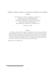
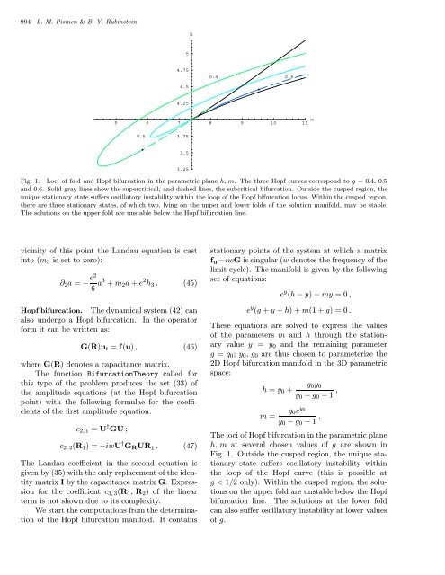
994 L. M. Pismen & B. Y. Rubinstein h 5 4.75 4.5 0.4 0.6 4.25 5 6 7 8 9 10 11 m 0.5 3.75 3.5 3.25 Fig. 1. Loci of fold and Hopf bifurcation in the parametric plane h, m. The three Hopf curves correspond to g =0.4, 0.5 and 0.6. Solid gray lines show the supercritical, and dashed lines, the subcritical bifurcation. Outside the cusped region, the unique stationary state suffers oscillatory instability within the loop of the Hopf bifurcation locus. Within the cusped region, there are three stationary states, of which two, lying on the upper and lower folds of the solution manifold, may be stable. The solutions on the upper fold are unstable below the Hopf bifurcation line. vicinity of this point the Landau equation is cast into (m 3 is set to zero): ∂ 2 a = − e2 6 a3 + m 2 a + e 2 h 3 . (45) Hopf bifurcation. The dynamical system (42) can also undergo a Hopf bifurcation. In the operator form it can be written as: G(R)u t = f(u) , (46) where G(R) denotes a capacitance matrix. The function BifurcationTheory called for this type of the problem produces the set (33) of the amplitude equations (at the Hopf bifurcation point) with the following formulae for the coefficients of the first amplitude equation: c 2, 1 = U † GU ; c 2, 2 (R 1 )=−iwU † G R UR 1 . (47) The Landau coefficient in the second equation is given by (35) with the only replacement of the identity matrix I by the capacitance matrix G. Expression for the coefficient c 3, 3 (R 1 , R 2 ) of the linear term is not shown due to its complexity. We start the computations from the determination of the Hopf bifurcation manifold. It contains stationary points of the system at which a matrix f u −iwG is singular (w denotes the frequency of the limit cycle). The manifold is given by the following set of equations: e y (h − y) − my =0, e y (g+y−h)+m(1 + g) =0. These equations are solved to express the values of the parameters m and h through the stationary value y = y 0 and the remaining parameter g = g 0 ; y 0 ,g 0 are thus chosen to parameterize the 2D Hopf bifurcation manifold in the 3D parametric space: h = y 0 + g 0 y 0 y 0 − g 0 − 1 , g 0 e y 0 m = y 0 − g 0 − 1 . The loci of Hopf bifurcation in the parametric plane h, m at several chosen values of g are shown in Fig. 1. Outside the cusped region, the unique stationary state suffers oscillatory instability within the loop of the Hopf curve (this is possible at g
Computer Tools for Bifurcation Analysis 995 Now it is possible to compute the frequency w = e y √ 0 y 0 − g 0 y 0 − 1/(1 + g 0 − y 0 )andtheeigenvectors: { g(1 − y0 − i √ } y 0 − g 0 y 0 − 1) U = , 1 ; y 0 (y 0 −1) y0 4 3.5 3 super sub U † = { (y 0 − 1) g 0(1 − y 0 + i √ } y 0 − g 0 y 0 − 1) ,1 1+g 0 −y 0 . (48) 2.5 2 1.5 1 0.5 sub As it was done above, one can choose the parametric deviation of the first-order in such a way as to make the first amplitude equation trivial. Then the Landau coefficient in the second equation can be presented after normalization as: c 3, 2 /c 3, 1 =(y 0 −g 0 y 0 −1) 3/2 (iy 0 − i − √ y 0 − g 0 y 0 − 1) −1 e y 0 /12 × (12 − 24g 0 − 24y 0 +40g 0 y 0 −4g 2 0 y 0 +14y 2 0−21g 0 y 2 0 +4g 2 0y 2 0 −2y 3 0 +2g 0 y 3 0 +i √ y 0 −g 0 y 0 −1(−12 + 24g 0 +15y 0 −25g 0 y 0 − 2g 2 0 y 0 − 5y 2 0 +8g 0y 2 0 )) . (49) 0 0.1 0.2 0.3 0.4 0.5 0.6 0.7 Fig. 2. The stability boundary in the plane (g 0,y 0), separating the regions of subcritical and supercritical Hopf bifurcation. The unphysical part of the curve below the boundary of positive frequency is shown by a dashed line. The solid circle at g 0 =0.5,y 0= 2 marks the double zero point. the unphysical part of the curve dipping below the boundary of positive frequency is shown by a dashed line. The region of subcritical bifurcations consists of two disconnected parts, of which the lower one lies within the region of unique stationary states and on the lower fold of the solution manifold, and the upper one, on the upper fold in the region of multiple solutions. g0 First, we take note that only a part of the parametric plane y 0 ,g 0 above the thick solid curve in Fig. 2 is actually available, since the condition of positive oscillation frequency requires y 0 − g 0 y 0 − 1 > 0 . (50) Within this region, the limit cycle is stable (the bifurcation is supercritical ) if the real part of the coefficient at the nonlinear term is negative. Extracting the real part from (49) brings this condition to the form 3g 0 +2g 2 0 +2y 0−4g 0 y 0 −2g 2 0 y 0−y 2 0 +2g 0y 2 0 −1 4(y 0 − 1 − g 0 )(y 0 − g 0 y 0 − 1) < 0 . (51) Noting that the denominator of the above fraction is positive whenever the inequality (50) is verified, one can determine the stability boundary by equating the numerator in (51) to zero, and combining the result with (50). The stability boundary in the plane (g 0 ,y 0 ), separating the regions of subcritical and supercritical bifurcation is shown in Fig. 2; 3. General Algorithm for Distributed Systems 3.1. Introduction The main point of our approach can be formulated as follows. An algorithm applicable to the nonlinear analysis of a number of representative realistic problems must be as general as possible, i.e. it must be designed for classes of problems (say, dynamical problems, or reaction–diffusion type problems), or even better, it should embrace all problems which can be solved using standard methods of bifurcation expansion. It is clear that the generalization from particular problems to some class of such problems can be performed using an operator form of the problem. For example, all reaction–diffusion type problems can be presented in the following operator form: G(R) ∂ u(r, t)=D(R)(∇·∇)u(r,t) ∂t +f(u(r,t),R), (52)
Page 1 and 2: Tutorials and Reviews International
Page 3 and 4: Computer Tools for Bifurcation Anal
Page 11: Computer Tools for Bifurcation Anal
Page 21 and 22: There is also additional differenti

Computer Tools for Bifurcation Analysis: General Approach with

You also want an ePaper? Increase the reach of your titles

Delete template?

Save as template?